
DATA 644 (Bayesian Reasoning in Data Science): Assignment 1
Contents
DATA 644 (Bayesian Reasoning in Data Science): Assignment 1#
%pip install pymc pytensor
Requirement already satisfied: pymc in /usr/local/lib/python3.10/dist-packages (5.7.2)
Requirement already satisfied: pytensor in /usr/local/lib/python3.10/dist-packages (2.14.2)
Requirement already satisfied: arviz>=0.13.0 in /usr/local/lib/python3.10/dist-packages (from pymc) (0.15.1)
Requirement already satisfied: cachetools>=4.2.1 in /usr/local/lib/python3.10/dist-packages (from pymc) (5.3.2)
Requirement already satisfied: cloudpickle in /usr/local/lib/python3.10/dist-packages (from pymc) (2.2.1)
Requirement already satisfied: fastprogress>=0.2.0 in /usr/local/lib/python3.10/dist-packages (from pymc) (1.0.3)
Requirement already satisfied: numpy>=1.15.0 in /usr/local/lib/python3.10/dist-packages (from pymc) (1.25.2)
Requirement already satisfied: pandas>=0.24.0 in /usr/local/lib/python3.10/dist-packages (from pymc) (1.5.3)
Requirement already satisfied: scipy>=1.4.1 in /usr/local/lib/python3.10/dist-packages (from pymc) (1.11.4)
Requirement already satisfied: typing-extensions>=3.7.4 in /usr/local/lib/python3.10/dist-packages (from pymc) (4.9.0)
Requirement already satisfied: setuptools>=48.0.0 in /usr/local/lib/python3.10/dist-packages (from pytensor) (67.7.2)
Requirement already satisfied: filelock in /usr/local/lib/python3.10/dist-packages (from pytensor) (3.13.1)
Requirement already satisfied: etuples in /usr/local/lib/python3.10/dist-packages (from pytensor) (0.3.9)
Requirement already satisfied: logical-unification in /usr/local/lib/python3.10/dist-packages (from pytensor) (0.4.6)
Requirement already satisfied: miniKanren in /usr/local/lib/python3.10/dist-packages (from pytensor) (1.0.3)
Requirement already satisfied: cons in /usr/local/lib/python3.10/dist-packages (from pytensor) (0.4.6)
Requirement already satisfied: matplotlib>=3.2 in /usr/local/lib/python3.10/dist-packages (from arviz>=0.13.0->pymc) (3.7.1)
Requirement already satisfied: packaging in /usr/local/lib/python3.10/dist-packages (from arviz>=0.13.0->pymc) (23.2)
Requirement already satisfied: xarray>=0.21.0 in /usr/local/lib/python3.10/dist-packages (from arviz>=0.13.0->pymc) (2023.7.0)
Requirement already satisfied: h5netcdf>=1.0.2 in /usr/local/lib/python3.10/dist-packages (from arviz>=0.13.0->pymc) (1.3.0)
Requirement already satisfied: xarray-einstats>=0.3 in /usr/local/lib/python3.10/dist-packages (from arviz>=0.13.0->pymc) (0.7.0)
Requirement already satisfied: python-dateutil>=2.8.1 in /usr/local/lib/python3.10/dist-packages (from pandas>=0.24.0->pymc) (2.8.2)
Requirement already satisfied: pytz>=2020.1 in /usr/local/lib/python3.10/dist-packages (from pandas>=0.24.0->pymc) (2023.4)
Requirement already satisfied: toolz in /usr/local/lib/python3.10/dist-packages (from logical-unification->pytensor) (0.12.1)
Requirement already satisfied: multipledispatch in /usr/local/lib/python3.10/dist-packages (from logical-unification->pytensor) (1.0.0)
Requirement already satisfied: h5py in /usr/local/lib/python3.10/dist-packages (from h5netcdf>=1.0.2->arviz>=0.13.0->pymc) (3.9.0)
Requirement already satisfied: contourpy>=1.0.1 in /usr/local/lib/python3.10/dist-packages (from matplotlib>=3.2->arviz>=0.13.0->pymc) (1.2.0)
Requirement already satisfied: cycler>=0.10 in /usr/local/lib/python3.10/dist-packages (from matplotlib>=3.2->arviz>=0.13.0->pymc) (0.12.1)
Requirement already satisfied: fonttools>=4.22.0 in /usr/local/lib/python3.10/dist-packages (from matplotlib>=3.2->arviz>=0.13.0->pymc) (4.48.1)
Requirement already satisfied: kiwisolver>=1.0.1 in /usr/local/lib/python3.10/dist-packages (from matplotlib>=3.2->arviz>=0.13.0->pymc) (1.4.5)
Requirement already satisfied: pillow>=6.2.0 in /usr/local/lib/python3.10/dist-packages (from matplotlib>=3.2->arviz>=0.13.0->pymc) (9.4.0)
Requirement already satisfied: pyparsing>=2.3.1 in /usr/local/lib/python3.10/dist-packages (from matplotlib>=3.2->arviz>=0.13.0->pymc) (3.1.1)
Requirement already satisfied: six>=1.5 in /usr/local/lib/python3.10/dist-packages (from python-dateutil>=2.8.1->pandas>=0.24.0->pymc) (1.16.0)
%matplotlib inline
import warnings

import arviz as az
import matplotlib as mpl
import matplotlib.pyplot as plt
import numpy as np
import pymc as pm
#import theano.tensor as tt

from pymc import Model, Normal, Slice, sample, HalfNormal
from pymc.distributions import Interpolated
from scipy import stats
#from theano import as_op

import pickle
from google.colab import files
import pickle

uploaded = files.upload()
Saving my_arrays.pkl to my_arrays.pkl
with open("my_arrays.pkl", 'rb') as file:
    data = pickle.load(file)
import numpy as np
np.shape(data['X1'])
(1000,)
X1 = data['X1']
X2 = data['X2']
Y = data['Y']
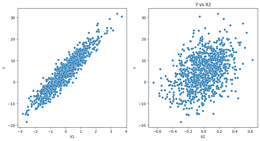
Visual inspection#
import pandas as pd
import statsmodels.api as sm
import seaborn as sns


# Create a DataFrame from the arrays
data = pd.DataFrame({
    'X1': X1,
    'X2': X2,
    'Y': Y
})

# Prepare the features and target variable
X = data[['X1', 'X2']]
X = sm.add_constant(X)  # Adds a constant term to the predictor
Y = data['Y']


# Visualization
plt.figure(figsize=(12, 6))

# Plot Y vs X1
plt.subplot(1, 2, 1)
sns.scatterplot(x='X1', y='Y', data=data)


# Plot Y vs X2
plt.subplot(1, 2, 2)
sns.scatterplot(x='X2', y='Y', data=data)

plt.title('Y vs X2')

plt.show()


#---- you can also do a linear fit, etc. (complete)

# Perform linear regression
model = sm.OLS(Y, X).fit()

# Print the summary to inspect the coefficients and model performance
print(model.summary())
                            OLS Regression Results
==============================================================================
Dep. Variable:                      Y   R-squared:                       0.984
Model:                            OLS   Adj. R-squared:                  0.984
Method:                 Least Squares   F-statistic:                 3.081e+04
Date:                Tue, 20 Feb 2024   Prob (F-statistic):               0.00
Time:                        15:21:11   Log-Likelihood:                -1395.6
No. Observations:                1000   AIC:                             2797.
Df Residuals:                     997   BIC:                             2812.
Df Model:                           2
Covariance Type:            nonrobust
==============================================================================
                 coef    std err          t      P>|t|      [0.025      0.975]
------------------------------------------------------------------------------
const          5.0115      0.031    161.944      0.000       4.951       5.072
X1             7.0540      0.031    229.558      0.000       6.994       7.114
X2            12.8148      0.155     82.457      0.000      12.510      13.120
==============================================================================
Omnibus:                        0.260   Durbin-Watson:                   2.042
Prob(Omnibus):                  0.878   Jarque-Bera (JB):                0.335
Skew:                          -0.027   Prob(JB):                        0.846
Kurtosis:                       2.929   Cond. No.                         5.10
==============================================================================

Notes:
[1] Standard Errors assume that the covariance matrix of the errors is correctly specified.
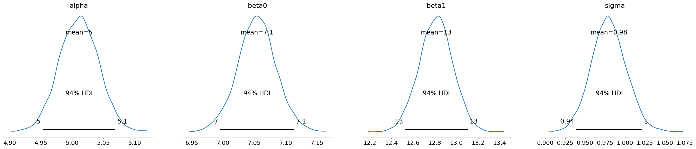
Building the Model#
basic_model = Model()

with basic_model:
    # Priors for unknown model parameters
    alpha = Normal("alpha", mu=0, sigma=10)
    beta0 = Normal("beta0", mu=0, sigma=10)
    beta1 = Normal("beta1", mu=0, sigma=10)
    sigma = HalfNormal("sigma",sigma=5)


    # Expected value of outcome
    mu = alpha + beta0 * X1 + beta1 * X2

    # Likelihood (sampling distribution) of observations
    Y_obs = Normal("Y_obs", mu=mu, sigma=sigma, observed=Y)

    # draw 1000 posterior samples
    trace_in = sample(5000)
100.00% [6000/6000 00:07<00:00 Sampling chain 0, 0 divergences]
100.00% [6000/6000 00:06<00:00 Sampling chain 1, 0 divergences]
az.plot_posterior(trace_in)
/usr/local/lib/python3.10/dist-packages/arviz/utils.py:184: NumbaDeprecationWarning: The 'nopython' keyword argument was not supplied to the 'numba.jit' decorator. The implicit default value for this argument is currently False, but it will be changed to True in Numba 0.59.0. See https://numba.readthedocs.io/en/stable/reference/deprecation.html#deprecation-of-object-mode-fall-back-behaviour-when-using-jit for details.
  numba_fn = numba.jit(**self.kwargs)(self.function)
array([<Axes: title={'center': 'alpha'}>,
       <Axes: title={'center': 'beta0'}>,
       <Axes: title={'center': 'beta1'}>,
       <Axes: title={'center': 'sigma'}>], dtype=object)
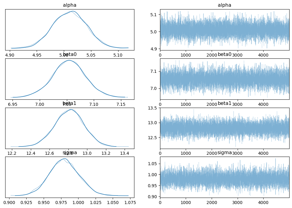
az.plot_trace(trace_in, compact=True)
array([[<Axes: title={'center': 'alpha'}>,
        <Axes: title={'center': 'alpha'}>],
       [<Axes: title={'center': 'beta0'}>,
        <Axes: title={'center': 'beta0'}>],
       [<Axes: title={'center': 'beta1'}>,
        <Axes: title={'center': 'beta1'}>],
       [<Axes: title={'center': 'sigma'}>,
        <Axes: title={'center': 'sigma'}>]], dtype=object)
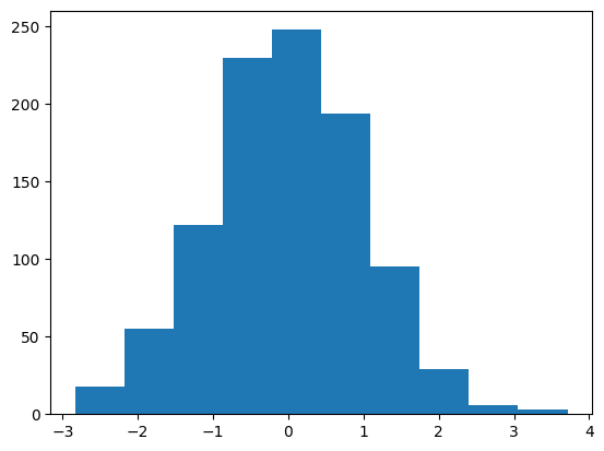
np.shape(X1)
(1000,)
plt.hist(X1)
(array([ 18.,  55., 122., 230., 248., 194.,  95.,  29.,   6.,   3.]),
 array([-2.83591463, -2.18122708, -1.52653953, -0.87185197, -0.21716442,
         0.43752313,  1.09221068,  1.74689823,  2.40158578,  3.05627333,
         3.71096089]),
 <BarContainer object of 10 artists>)
az.summary(trace_in,hdi_prob=0.94)
| mean | sd | hdi_3% | hdi_97% | mcse_mean | mcse_sd | ess_bulk | ess_tail | r_hat | |
|---|---|---|---|---|---|---|---|---|---|
| alpha | 5.011 | 0.031 | 4.953 | 5.069 | 0.000 | 0.000 | 17161.0 | 7772.0 | 1.0 |
| beta0 | 7.054 | 0.031 | 6.995 | 7.114 | 0.000 | 0.000 | 15873.0 | 8126.0 | 1.0 |
| beta1 | 12.811 | 0.154 | 12.525 | 13.103 | 0.001 | 0.001 | 14779.0 | 8785.0 | 1.0 |
| sigma | 0.980 | 0.022 | 0.939 | 1.021 | 0.000 | 0.000 | 11961.0 | 8264.0 | 1.0 |
What happens if using 10 observations only?#
# Generate 10 random unique indices from the range of your data length
random_indices = np.random.choice(len(X1), 10, replace=False)


# Select the corresponding elements from X1, X2, and Y
selected_X1 = X1[random_indices]
selected_X2 = X2[random_indices]
selected_Y = Y.values[random_indices]
selected_model = Model()

with selected_model:
    # Priors for unknown model parameters
    alpha = Normal("alpha", mu=0, sigma=10)
    beta0 = Normal("beta0", mu=0, sigma=10)
    beta1 = Normal("beta1", mu=0, sigma=10)
    sigma = HalfNormal("sigma",sigma=5)


    # Expected value of outcome
    mu = alpha + beta0 * selected_X1 + beta1 * selected_X2

    # Likelihood (sampling distribution) of observations
    Y_obs = Normal("Y_obs", mu=mu, sigma=sigma, observed=selected_Y)

    # draw 1000 posterior samples
    trace_selected = sample(5000)
100.00% [6000/6000 00:08<00:00 Sampling chain 0, 1 divergences]
100.00% [6000/6000 00:09<00:00 Sampling chain 1, 0 divergences]
az.plot_posterior(trace_selected)
array([<Axes: title={'center': 'alpha'}>,
       <Axes: title={'center': 'beta0'}>,
       <Axes: title={'center': 'beta1'}>,
       <Axes: title={'center': 'sigma'}>], dtype=object)
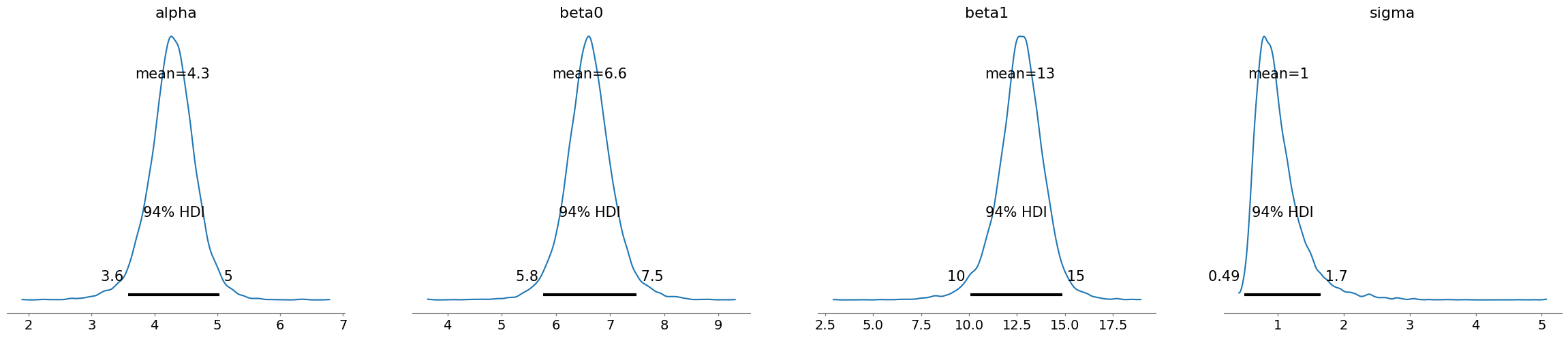
az.summary(trace_selected,hdi_prob=0.94)
| mean | sd | hdi_3% | hdi_97% | mcse_mean | mcse_sd | ess_bulk | ess_tail | r_hat | |
|---|---|---|---|---|---|---|---|---|---|
| alpha | 4.283 | 0.385 | 3.581 | 5.033 | 0.005 | 0.004 | 6071.0 | 4790.0 | 1.0 |
| beta0 | 6.620 | 0.453 | 5.761 | 7.487 | 0.006 | 0.004 | 6391.0 | 4463.0 | 1.0 |
| beta1 | 12.654 | 1.270 | 10.052 | 14.876 | 0.017 | 0.012 | 5998.0 | 4707.0 | 1.0 |
| sigma | 1.006 | 0.370 | 0.493 | 1.653 | 0.006 | 0.004 | 3700.0 | 4565.0 | 1.0 |
The HDI intervals become broader, highlighting more uncertainty (less observations means less information we could leverage on in our model)