Logistic Regression

%pip install pytensor pymc

Requirement already satisfied: pytensor in /usr/local/lib/python3.10/dist-packages (2.14.2)
Requirement already satisfied: pymc in /usr/local/lib/python3.10/dist-packages (5.7.2)
Requirement already satisfied: setuptools>=48.0.0 in /usr/local/lib/python3.10/dist-packages (from pytensor) (67.7.2)
Requirement already satisfied: scipy>=0.14 in /usr/local/lib/python3.10/dist-packages (from pytensor) (1.11.4)
Requirement already satisfied: numpy>=1.17.0 in /usr/local/lib/python3.10/dist-packages (from pytensor) (1.25.2)
Requirement already satisfied: filelock in /usr/local/lib/python3.10/dist-packages (from pytensor) (3.13.1)
Requirement already satisfied: etuples in /usr/local/lib/python3.10/dist-packages (from pytensor) (0.3.9)
Requirement already satisfied: logical-unification in /usr/local/lib/python3.10/dist-packages (from pytensor) (0.4.6)
Requirement already satisfied: miniKanren in /usr/local/lib/python3.10/dist-packages (from pytensor) (1.0.3)
Requirement already satisfied: cons in /usr/local/lib/python3.10/dist-packages (from pytensor) (0.4.6)
Requirement already satisfied: typing-extensions in /usr/local/lib/python3.10/dist-packages (from pytensor) (4.9.0)
Requirement already satisfied: arviz>=0.13.0 in /usr/local/lib/python3.10/dist-packages (from pymc) (0.15.1)
Requirement already satisfied: cachetools>=4.2.1 in /usr/local/lib/python3.10/dist-packages (from pymc) (5.3.2)
Requirement already satisfied: cloudpickle in /usr/local/lib/python3.10/dist-packages (from pymc) (2.2.1)
Requirement already satisfied: fastprogress>=0.2.0 in /usr/local/lib/python3.10/dist-packages (from pymc) (1.0.3)
Requirement already satisfied: pandas>=0.24.0 in /usr/local/lib/python3.10/dist-packages (from pymc) (1.5.3)
Requirement already satisfied: matplotlib>=3.2 in /usr/local/lib/python3.10/dist-packages (from arviz>=0.13.0->pymc) (3.7.1)
Requirement already satisfied: packaging in /usr/local/lib/python3.10/dist-packages (from arviz>=0.13.0->pymc) (23.2)
Requirement already satisfied: xarray>=0.21.0 in /usr/local/lib/python3.10/dist-packages (from arviz>=0.13.0->pymc) (2023.7.0)
Requirement already satisfied: h5netcdf>=1.0.2 in /usr/local/lib/python3.10/dist-packages (from arviz>=0.13.0->pymc) (1.3.0)
Requirement already satisfied: xarray-einstats>=0.3 in /usr/local/lib/python3.10/dist-packages (from arviz>=0.13.0->pymc) (0.7.0)
Requirement already satisfied: python-dateutil>=2.8.1 in /usr/local/lib/python3.10/dist-packages (from pandas>=0.24.0->pymc) (2.8.2)
Requirement already satisfied: pytz>=2020.1 in /usr/local/lib/python3.10/dist-packages (from pandas>=0.24.0->pymc) (2023.4)
Requirement already satisfied: toolz in /usr/local/lib/python3.10/dist-packages (from logical-unification->pytensor) (0.12.1)
Requirement already satisfied: multipledispatch in /usr/local/lib/python3.10/dist-packages (from logical-unification->pytensor) (1.0.0)
Requirement already satisfied: h5py in /usr/local/lib/python3.10/dist-packages (from h5netcdf>=1.0.2->arviz>=0.13.0->pymc) (3.9.0)
Requirement already satisfied: contourpy>=1.0.1 in /usr/local/lib/python3.10/dist-packages (from matplotlib>=3.2->arviz>=0.13.0->pymc) (1.2.0)
Requirement already satisfied: cycler>=0.10 in /usr/local/lib/python3.10/dist-packages (from matplotlib>=3.2->arviz>=0.13.0->pymc) (0.12.1)
Requirement already satisfied: fonttools>=4.22.0 in /usr/local/lib/python3.10/dist-packages (from matplotlib>=3.2->arviz>=0.13.0->pymc) (4.49.0)
Requirement already satisfied: kiwisolver>=1.0.1 in /usr/local/lib/python3.10/dist-packages (from matplotlib>=3.2->arviz>=0.13.0->pymc) (1.4.5)
Requirement already satisfied: pillow>=6.2.0 in /usr/local/lib/python3.10/dist-packages (from matplotlib>=3.2->arviz>=0.13.0->pymc) (9.4.0)
Requirement already satisfied: pyparsing>=2.3.1 in /usr/local/lib/python3.10/dist-packages (from matplotlib>=3.2->arviz>=0.13.0->pymc) (3.1.1)
Requirement already satisfied: six>=1.5 in /usr/local/lib/python3.10/dist-packages (from python-dateutil>=2.8.1->pandas>=0.24.0->pymc) (1.16.0)

import pymc as pm
import numpy as np
import pandas as pd
import seaborn as sns
import scipy.stats as stats
from scipy.special import expit as logistic
import matplotlib.pyplot as plt
import arviz as az
import requests
import io

az.style.use('arviz-darkgrid')

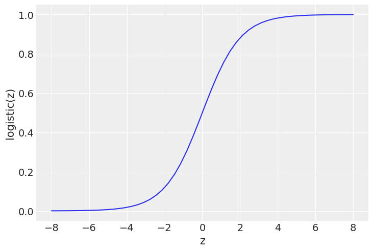
z = np.linspace(-8, 8)
plt.plot(z, 1 / (1 + np.exp(-z)))
plt.xlabel('z')
plt.ylabel('logistic(z)')

Text(0, 0.5, 'logistic(z)')

The Iris Dataset

target_url = 'https://raw.githubusercontent.com/cfteach/brds/main/datasets/iris.csv'

download = requests.get(target_url).content
iris = pd.read_csv(io.StringIO(download.decode('utf-8')))

iris.head()

	sepal_length	sepal_width	petal_length	petal_width	species
0	5.1	3.5	1.4	0.2	setosa
1	4.9	3.0	1.4	0.2	setosa
2	4.7	3.2	1.3	0.2	setosa
3	4.6	3.1	1.5	0.2	setosa
4	5.0	3.6	1.4	0.2	setosa

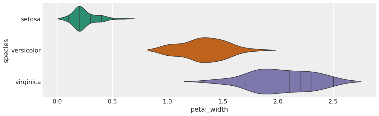
# @title species vs petal_width

from matplotlib import pyplot as plt
import seaborn as sns
figsize = (12, 1.2 * len(iris['species'].unique()))
plt.figure(figsize=figsize)
sns.violinplot(iris, x='petal_width', y='species', inner='stick', palette='Dark2')
sns.despine(top=True, right=True, bottom=True, left=True)

<ipython-input-6-7a5e472054ba>:7: FutureWarning: 

Passing `palette` without assigning `hue` is deprecated and will be removed in v0.14.0. Assign the `y` variable to `hue` and set `legend=False` for the same effect.

  sns.violinplot(iris, x='petal_width', y='species', inner='stick', palette='Dark2')

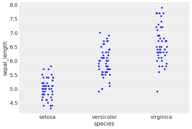
#using stripplot function from seaborn

sns.stripplot(x="species", y="sepal_length", data=iris, jitter=True)

<Axes: xlabel='species', ylabel='sepal_length'>

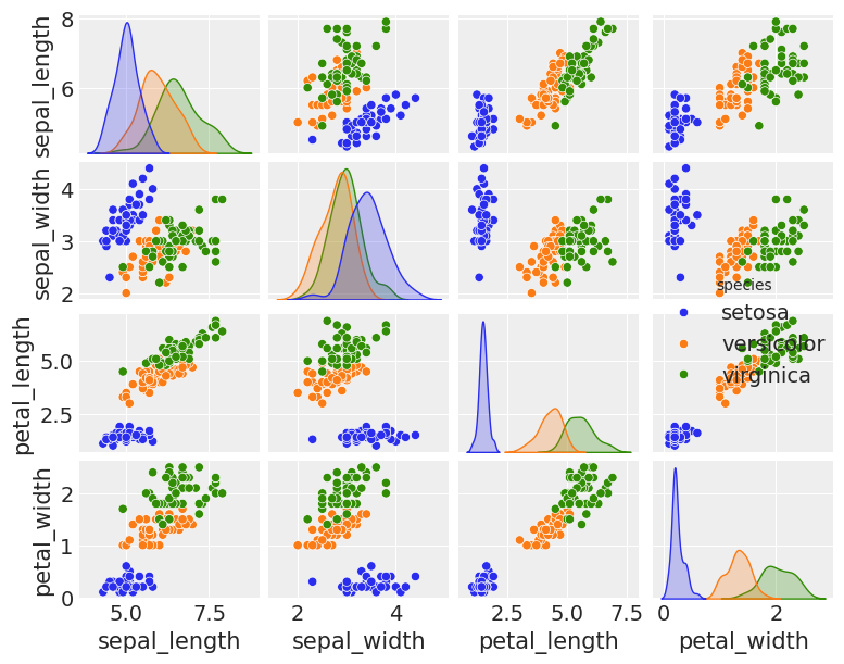
sns.pairplot(iris, hue='species', diag_kind='kde', height=1.5)

/usr/local/lib/python3.10/dist-packages/seaborn/axisgrid.py:123: UserWarning: The figure layout has changed to tight
  self._figure.tight_layout(*args, **kwargs)
/usr/local/lib/python3.10/dist-packages/seaborn/axisgrid.py:213: UserWarning: This figure was using a layout engine that is incompatible with subplots_adjust and/or tight_layout; not calling subplots_adjust.
  self._figure.subplots_adjust(right=right)
/usr/local/lib/python3.10/dist-packages/seaborn/axisgrid.py:123: UserWarning: The figure layout has changed to tight
  self._figure.tight_layout(*args, **kwargs)

<seaborn.axisgrid.PairGrid at 0x7eb08ed760b0>

The logistic model applied to the iris dataset

df = iris.query("species == ('setosa', 'versicolor')")

df

	sepal_length	sepal_width	petal_length	petal_width	species
0	5.1	3.5	1.4	0.2	setosa
1	4.9	3.0	1.4	0.2	setosa
2	4.7	3.2	1.3	0.2	setosa
3	4.6	3.1	1.5	0.2	setosa
4	5.0	3.6	1.4	0.2	setosa
...	...	...	...	...	...
95	5.7	3.0	4.2	1.2	versicolor
96	5.7	2.9	4.2	1.3	versicolor
97	6.2	2.9	4.3	1.3	versicolor
98	5.1	2.5	3.0	1.1	versicolor
99	5.7	2.8	4.1	1.3	versicolor

100 rows × 5 columns

# converting the 'species' column of a DataFrame df into categorical codes using Pandas
y_0 = pd.Categorical(df['species']).codes

y_0

array([0, 0, 0, 0, 0, 0, 0, 0, 0, 0, 0, 0, 0, 0, 0, 0, 0, 0, 0, 0, 0, 0,
       0, 0, 0, 0, 0, 0, 0, 0, 0, 0, 0, 0, 0, 0, 0, 0, 0, 0, 0, 0, 0, 0,
       0, 0, 0, 0, 0, 0, 1, 1, 1, 1, 1, 1, 1, 1, 1, 1, 1, 1, 1, 1, 1, 1,
       1, 1, 1, 1, 1, 1, 1, 1, 1, 1, 1, 1, 1, 1, 1, 1, 1, 1, 1, 1, 1, 1,
       1, 1, 1, 1, 1, 1, 1, 1, 1, 1, 1, 1], dtype=int8)

# let's select one variate
x_n = 'sepal_length'
x_0 = df[x_n].values
#print(x_0)

# let's center our dataset, as we have done in other exercises
x_c = x_0 - x_0.mean()
print(x_c)

[-0.371 -0.571 -0.771 -0.871 -0.471 -0.071 -0.871 -0.471 -1.071 -0.571
 -0.071 -0.671 -0.671 -1.171  0.329  0.229 -0.071 -0.371  0.229 -0.371
 -0.071 -0.371 -0.871 -0.371 -0.671 -0.471 -0.471 -0.271 -0.271 -0.771
 -0.671 -0.071 -0.271  0.029 -0.571 -0.471  0.029 -0.571 -1.071 -0.371
 -0.471 -0.971 -1.071 -0.471 -0.371 -0.671 -0.371 -0.871 -0.171 -0.471
  1.529  0.929  1.429  0.029  1.029  0.229  0.829 -0.571  1.129 -0.271
 -0.471  0.429  0.529  0.629  0.129  1.229  0.129  0.329  0.729  0.129
  0.429  0.629  0.829  0.629  0.929  1.129  1.329  1.229  0.529  0.229
  0.029  0.029  0.329  0.529 -0.071  0.529  1.229  0.829  0.129  0.029
  0.029  0.629  0.329 -0.471  0.129  0.229  0.229  0.729 -0.371  0.229]

with pm.Model() as model_logreg:
    α = pm.Normal('α', mu=0, sigma=10)
    β = pm.Normal('β', mu=0, sigma=10)

    #μ = α + pm.math.dot(x_c, β)
    μ = α + β * x_c
    θ = pm.Deterministic('θ', pm.math.sigmoid(μ))
    bd = pm.Deterministic('bd', -α/β)

    yl = pm.Bernoulli('yl', p=θ, observed=y_0)

    idata_logreg = pm.sample(2000, tune = 2000, return_inferencedata=True)

100.00% [4000/4000 00:03<00:00 Sampling chain 0, 0 divergences]

100.00% [4000/4000 00:04<00:00 Sampling chain 1, 0 divergences]

varnames = ['α', 'β', 'bd']
res = az.summary(idata_logreg)
#print(res)
az.summary(idata_logreg)

/usr/local/lib/python3.10/dist-packages/arviz/utils.py:184: NumbaDeprecationWarning: The 'nopython' keyword argument was not supplied to the 'numba.jit' decorator. The implicit default value for this argument is currently False, but it will be changed to True in Numba 0.59.0. See https://numba.readthedocs.io/en/stable/reference/deprecation.html#deprecation-of-object-mode-fall-back-behaviour-when-using-jit for details.
  numba_fn = numba.jit(**self.kwargs)(self.function)

	mean	sd	hdi_3%	hdi_97%	mcse_mean	mcse_sd	ess_bulk	ess_tail	r_hat
α	0.307	0.337	-0.324	0.930	0.006	0.004	3606.0	2730.0	1.0
β	5.405	1.049	3.559	7.453	0.018	0.013	3428.0	2575.0	1.0
θ[0]	0.163	0.059	0.067	0.280	0.001	0.001	3901.0	2762.0	1.0
θ[1]	0.067	0.036	0.012	0.136	0.001	0.000	3722.0	2779.0	1.0
θ[2]	0.027	0.020	0.001	0.064	0.000	0.000	3630.0	2741.0	1.0
...	...	...	...	...	...	...	...	...	...
θ[96]	0.815	0.066	0.698	0.937	0.001	0.001	3295.0	2457.0	1.0
θ[97]	0.980	0.018	0.948	1.000	0.000	0.000	3249.0	2327.0	1.0
θ[98]	0.163	0.059	0.067	0.280	0.001	0.001	3901.0	2762.0	1.0
θ[99]	0.815	0.066	0.698	0.937	0.001	0.001	3295.0	2457.0	1.0
bd	-0.056	0.062	-0.168	0.067	0.001	0.001	3462.0	2690.0	1.0

103 rows × 9 columns

theta_post= idata_logreg.posterior['θ']
print(np.shape(theta_post))

(2, 2000, 100)

theta = idata_logreg.posterior['θ'].mean(axis=0).mean(axis=0)
idx = np.argsort(x_c)

np.random.seed(123)

# plotting the sigmoid (logistic) curve
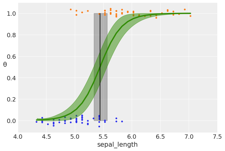
plt.plot(x_c[idx], theta[idx], color='C2', lw=3)

# plotting the mean boundary decision
plt.vlines(idata_logreg.posterior['bd'].mean(), 0, 1, color='k')

# ax.hdi will computer a lower and higher value of bd
bd_hdp = az.hdi(idata_logreg.posterior['bd'])

# Fill the area between two vertical curves.
plt.fill_betweenx([0, 1], bd_hdp.bd[0].values, bd_hdp.bd[1].values, color='k', alpha=0.25)


plt.scatter(x_c, np.random.normal(y_0, 0.02),
            marker='.', color=[f'C{x}' for x in y_0]) # 0.02 added for visualization purposes


az.plot_hdi(x_c, idata_logreg.posterior['θ'], color='C2')  #green band


plt.xlabel(x_n)
plt.ylabel('θ', rotation=0)
# use original scale for xticks
locs, _ = plt.xticks()
plt.xticks(locs, np.round(locs + x_0.mean(), 1))

([<matplotlib.axis.XTick at 0x7eb046565e10>,
  <matplotlib.axis.XTick at 0x7eb046565e40>,
  <matplotlib.axis.XTick at 0x7eb0465270d0>,
  <matplotlib.axis.XTick at 0x7eb0463d2d40>,
  <matplotlib.axis.XTick at 0x7eb0463d37f0>,
  <matplotlib.axis.XTick at 0x7eb0463fc2e0>,
  <matplotlib.axis.XTick at 0x7eb0463d3160>,
  <matplotlib.axis.XTick at 0x7eb0463fceb0>],
 [Text(-1.5, 0, '4.0'),
  Text(-1.0, 0, '4.5'),
  Text(-0.5, 0, '5.0'),
  Text(0.0, 0, '5.5'),
  Text(0.5, 0, '6.0'),
  Text(1.0, 0, '6.5'),
  Text(1.5, 0, '7.0'),
  Text(2.0, 0, '7.5')])

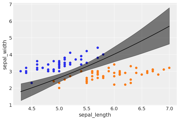
Multidimensional (feature space) Logistic Regression

df = iris.query("species == ('setosa', 'versicolor')")
y_1 = pd.Categorical(df['species']).codes
x_n = ['sepal_length', 'sepal_width']
x_1 = df[x_n].values

print(np.shape(x_1), type(x_1))
print(np.shape(y_1), type(y_1))

(100, 2) <class 'numpy.ndarray'>
(100,) <class 'numpy.ndarray'>

np.shape(x_1[:,0])

(100,)

with pm.Model() as model_1:

    α = pm.Normal('α', mu=0, sigma=10)
    β = pm.Normal('β', mu=0, sigma=2, shape=len(x_n))

    #Data container that registers a data variable with the model.
    #x__1 = pm.Data('x', x_1, mutable=True)
    #y__1 = pm.Data('y', y_1, mutable=True)
    # advantages: Model Reusability; Update Beliefs (reusing model); Efficeincy in sampling (same computational graph, even when data changes)
    #Depending on the mutable setting (default: True), the variable is registered as a SharedVariable, enabling it to be altered in value and shape, but NOT in dimensionality using pymc.set_data().

    μ = α + pm.math.dot(x_1, β)


    θ = pm.Deterministic('θ', 1 / (1 + pm.math.exp(-μ)))
    bd = pm.Deterministic('bd', -α/β[1] - β[0]/β[1] * x_1[:,0])



    yl = pm.Bernoulli('yl', p=θ, observed=y_1)

    trace_1 = pm.sample(1000, tune=2000, return_inferencedata=True, target_accept=0.9)

100.00% [3000/3000 00:26<00:00 Sampling chain 0, 0 divergences]

100.00% [3000/3000 00:24<00:00 Sampling chain 1, 0 divergences]

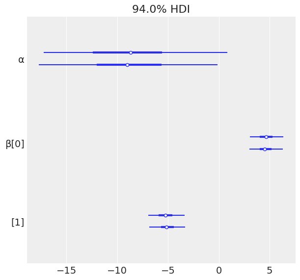
varnames = ['α', 'β']
az.plot_forest(trace_1, var_names=varnames);

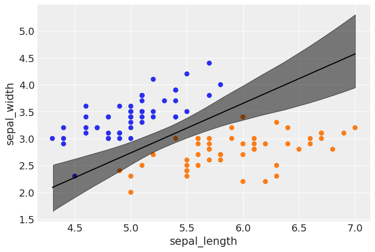
idx = np.argsort(x_1[:,0])


bd_mean = trace_1.posterior['bd'].mean(axis=0).mean(axis=0)


plt.scatter(x_1[:,0], x_1[:,1], c=[f'C{x}' for x in y_0])

bd = bd_mean[idx]

plt.plot(x_1[:,0][idx], bd, color='k');


az.plot_hdi(x_1[:,0], trace_1.posterior['bd'], color='k')


plt.xlabel(x_n[0])
plt.ylabel(x_n[1])

Text(0, 0.5, 'sepal_width')

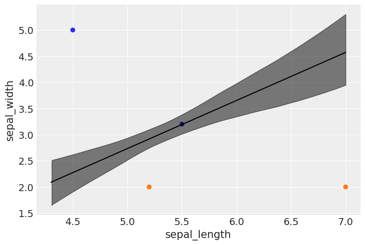
Prediction on unseen data

print(np.shape(x_1), type(x_1))

udata = np.array(((5.2,2.0),(7.0,2.0),(4.5,5.0),(5.5,3.2)))

print(np.shape(udata), type(udata))

(100, 2) <class 'numpy.ndarray'>
(4, 2) <class 'numpy.ndarray'>

print(udata)

[[5.2 2. ]
 [7.  2. ]
 [4.5 5. ]
 [5.5 3.2]]

alpha_chain = trace_1.posterior['α'].mean(axis=0).values
beta_chain  = trace_1.posterior['β'].mean(axis=0).values

print(np.shape(alpha_chain), np.shape(beta_chain))

(1000,) (1000, 2)

logit = np.dot(udata, beta_chain.T) + alpha_chain
print(np.shape(logit))

(4, 1000)

probabilities = 1 / (1 + np.exp(-logit))
print(np.shape(probabilities))

(4, 1000)

# Average probabilities for prediction
mean_probabilities = np.mean(probabilities, axis=1)

# Class assignment (you might adjust the threshold if needed, default is 0.5)
class_assignments = (mean_probabilities > 0.5).astype(int)

# Uncertainty estimation
lower_bound = np.percentile(probabilities, 2.5, axis=1)
upper_bound = np.percentile(probabilities, 97.5, axis=1)

print("\n=======================================")
print("data: \n", udata.T)
print("class, probabilities, ranges(94%HDI): ")
for h,i,j,k in zip(class_assignments, mean_probabilities, lower_bound,upper_bound):
  print(f"class: {h}, mean prob. {i:.4f}, 94% HDI: [{j:.4f},{k:.4f}]")

print("=======================================\n")

=======================================
data: 
 [[5.2 7.  4.5 5.5]
 [2.  2.  5.  3.2]]
class, probabilities, ranges(94%HDI): 
class: 1, mean prob. 0.9890, 94% HDI: [0.9652,0.9980]
class: 1, mean prob. 1.0000, 94% HDI: [1.0000,1.0000]
class: 0, mean prob. 0.0000, 94% HDI: [0.0000,0.0000]
class: 0, mean prob. 0.4861, 94% HDI: [0.3234,0.6602]
=======================================

bd_mean = trace_1.posterior['bd'].mean(axis=0).mean(axis=0)


plt.scatter(udata[:,0], udata[:,1], c=[f'C{x}' for x in class_assignments])

bd = bd_mean[idx]

plt.plot(x_1[:,0][idx], bd, color='k');

az.plot_hdi(x_1[:,0], trace_1.posterior['bd'], color='k')

plt.xlabel(x_n[0])
plt.ylabel(x_n[1])

Text(0, 0.5, 'sepal_width')

np.shape(x_1**2)

(100, 2)

x_1sq = x_1**2
print(np.shape(x_1sq), np.shape(x_1))

(100, 2) (100, 2)

Can I use a non-linear decision boundary?

Let’s add, for example, a term \(\gamma \cdot x_{sepal \ length}^2\) in the equation for \(\mu\)

with pm.Model() as model_2:
    α = pm.Normal('α', mu=0, sigma=10)
    β = pm.Normal('β', mu=0, sigma=2, shape=len(x_n))
    𝛾 = pm.Normal('𝛾', mu=0, sigma=2)

    μ = α + pm.math.dot(x_1, β) + pm.math.dot(x_1[:,0]**2,𝛾)

    θ = pm.Deterministic('θ', 1 / (1 + pm.math.exp(-μ)))
    bd = pm.Deterministic('bd', -α/β[1] - β[0]/β[1] * x_1[:,0] - 𝛾/β[1] * x_1[:,0]**2)

    yl = pm.Bernoulli('yl', p=θ, observed=y_1)

    trace_2 = pm.sample(1000, tune=2000, return_inferencedata=True, target_accept=0.95)

100.00% [3000/3000 01:00<00:00 Sampling chain 0, 0 divergences]

100.00% [3000/3000 00:58<00:00 Sampling chain 1, 0 divergences]

trace_2

arviz.InferenceData

• posterior

  <xarray.Dataset>
  Dimensions:   (chain: 2, draw: 1000, β_dim_0: 2, θ_dim_0: 100, bd_dim_0: 100)
  Coordinates:
    * chain     (chain) int64 0 1
    * draw      (draw) int64 0 1 2 3 4 5 6 7 8 ... 992 993 994 995 996 997 998 999
    * β_dim_0   (β_dim_0) int64 0 1
    * θ_dim_0   (θ_dim_0) int64 0 1 2 3 4 5 6 7 8 9 ... 91 92 93 94 95 96 97 98 99
    * bd_dim_0  (bd_dim_0) int64 0 1 2 3 4 5 6 7 8 ... 91 92 93 94 95 96 97 98 99
  Data variables:
      α         (chain, draw) float64 1.62 -7.419 0.1927 ... 11.85 13.82 13.3
      β         (chain, draw, β_dim_0) float64 -2.621 -7.707 ... -1.832 -5.801
      𝛾         (chain, draw) float64 1.246 1.305 0.4872 ... 0.523 0.4905 0.4845
      θ         (chain, draw, θ_dim_0) float64 0.001814 0.01183 ... 0.8868 0.9136
      bd        (chain, draw, bd_dim_0) float64 2.681 2.426 2.183 ... 2.855 3.206
  Attributes:
      created_at:                 2024-02-22T19:31:16.798921
      arviz_version:              0.15.1
      inference_library:          pymc
      inference_library_version:  5.7.2
      sampling_time:              119.82878065109253
      tuning_steps:               2000

  xarray.Dataset

  • Dimensions:
    • chain: 2
    • draw: 1000
    • β_dim_0: 2
    • θ_dim_0: 100
    • bd_dim_0: 100
  • Coordinates: (5)
    • chain
      (chain)
      int64
      0 1

      array([0, 1])

    • draw
      (draw)
      int64
      0 1 2 3 4 5 ... 995 996 997 998 999

      array([  0,   1,   2, ..., 997, 998, 999])

    • β_dim_0
      (β_dim_0)
      int64
      0 1

      array([0, 1])

    • θ_dim_0
      (θ_dim_0)
      int64
      0 1 2 3 4 5 6 ... 94 95 96 97 98 99

      array([ 0,  1,  2,  3,  4,  5,  6,  7,  8,  9, 10, 11, 12, 13, 14, 15, 16, 17,
             18, 19, 20, 21, 22, 23, 24, 25, 26, 27, 28, 29, 30, 31, 32, 33, 34, 35,
             36, 37, 38, 39, 40, 41, 42, 43, 44, 45, 46, 47, 48, 49, 50, 51, 52, 53,
             54, 55, 56, 57, 58, 59, 60, 61, 62, 63, 64, 65, 66, 67, 68, 69, 70, 71,
             72, 73, 74, 75, 76, 77, 78, 79, 80, 81, 82, 83, 84, 85, 86, 87, 88, 89,
             90, 91, 92, 93, 94, 95, 96, 97, 98, 99])

    • bd_dim_0
      (bd_dim_0)
      int64
      0 1 2 3 4 5 6 ... 94 95 96 97 98 99

      array([ 0,  1,  2,  3,  4,  5,  6,  7,  8,  9, 10, 11, 12, 13, 14, 15, 16, 17,
             18, 19, 20, 21, 22, 23, 24, 25, 26, 27, 28, 29, 30, 31, 32, 33, 34, 35,
             36, 37, 38, 39, 40, 41, 42, 43, 44, 45, 46, 47, 48, 49, 50, 51, 52, 53,
             54, 55, 56, 57, 58, 59, 60, 61, 62, 63, 64, 65, 66, 67, 68, 69, 70, 71,
             72, 73, 74, 75, 76, 77, 78, 79, 80, 81, 82, 83, 84, 85, 86, 87, 88, 89,
             90, 91, 92, 93, 94, 95, 96, 97, 98, 99])

  • Data variables: (5)
    • α
      (chain, draw)
      float64
      1.62 -7.419 0.1927 ... 13.82 13.3

      array([[ 1.62028048, -7.41908776,  0.19271947, ...,  5.35628133,
              -3.75805757, -2.98553493],
             [-6.72903573, -0.73632503, -0.95386675, ..., 11.85056643,
              13.82046429, 13.3021922 ]])

    • β
      (chain, draw, β_dim_0)
      float64
      -2.621 -7.707 ... -1.832 -5.801

      array([[[-2.62097149, -7.70659048],
              [-0.62446558, -8.42410746],
              [ 0.02639577, -4.47793844],
              ...,
              [-2.6494536 , -5.83418285],
              [-0.26120234, -7.5904906 ],
              [ 2.70250932, -7.76138423]],
      
             [[ 2.71858886, -5.62893395],
              [ 0.34452053, -5.48822705],
              [-1.19430668, -5.04252567],
              ...,
              [-1.90408364, -5.55200053],
              [-1.85788088, -5.72630518],
              [-1.83199512, -5.800672  ]]])

    • 𝛾
      (chain, draw)
      float64
      1.246 1.305 ... 0.4905 0.4845

      array([[1.24603301, 1.30543502, 0.48719373, ..., 0.93120808, 0.96586956,
              0.39581023],
             [0.32355101, 0.54377206, 0.79543266, ..., 0.52296391, 0.49052144,
              0.48445421]])

    • θ
      (chain, draw, θ_dim_0)
      float64
      0.001814 0.01183 ... 0.8868 0.9136

      array([[[1.81396912e-03, 1.18325401e-02, 3.95681196e-04, ...,
               9.99981883e-01, 8.01575128e-01, 9.96263647e-01],
              [2.16347542e-03, 1.20353742e-02, 2.08750852e-04, ...,
               9.99999475e-01, 9.08064980e-01, 9.99609441e-01],
              [6.45530091e-02, 1.95566923e-01, 3.73084240e-02, ...,
               9.97757857e-01, 8.58683784e-01, 9.74266017e-01],
              ...,
              [1.26814833e-02, 5.89512673e-02, 5.51282960e-03, ...,
               9.99592954e-01, 8.14471823e-01, 9.84837247e-01],
              [1.45014682e-03, 9.76737027e-03, 3.56357449e-04, ...,
               9.99941010e-01, 7.41896931e-01, 9.92466380e-01],
              [2.29996636e-03, 2.86373416e-02, 1.69780003e-03, ...,
               9.98463873e-01, 8.44069713e-01, 9.71989530e-01]],
      
             [[1.55206809e-02, 7.40354217e-02, 8.02596645e-03, ...,
               9.98053177e-01, 8.14420649e-01, 9.71197793e-01],
              [1.72159400e-02, 7.89362693e-02, 9.30845323e-03, ...,
               9.98318593e-01, 8.09022843e-01, 9.71461858e-01],
              [1.79074751e-02, 5.54509676e-02, 5.86959396e-03, ...,
               9.99497061e-01, 7.38475195e-01, 9.81350682e-01],
              ...,
              [2.43642932e-02, 1.70925613e-01, 3.51361827e-02, ...,
               9.82828425e-01, 8.65533377e-01, 9.20032283e-01],
              [5.02907953e-02, 3.35224735e-01, 8.31624867e-02, ...,
               9.89553241e-01, 9.42022350e-01, 9.58270838e-01],
              [2.31422568e-02, 1.90794774e-01, 4.03591229e-02, ...,
               9.76894177e-01, 8.86752599e-01, 9.13556630e-01]]])

    • bd
      (chain, draw, bd_dim_0)
      float64
      2.681 2.426 2.183 ... 2.855 3.206

      array([[[2.68116548, 2.42581628, 2.18340181, ..., 4.31679431,
               2.68116548, 3.52482144],
              [2.77186666, 2.47676395, 2.19405838, ..., 4.61653034,
               2.77186666, 3.73155759],
              [2.90295344, 2.68417718, 2.47410482, ..., 4.26180494,
               2.90295344, 3.61150557],
              ...,
              [2.75356303, 2.52516336, 2.30953268, ..., 4.23800699,
               2.75356303, 3.51537601],
              [2.63910186, 2.39148958, 2.15405709, ..., 4.18293304,
               2.63910186, 3.4430174 ],
              [2.71759341, 2.54595878, 2.37840394, ..., 3.73451013,
               2.71759341, 3.25697604]],
      
             [[2.76274859, 2.55119524, 2.3442403 , ..., 4.00848835,
               2.76274859, 3.42499901],
              [2.76304913, 2.55233477, 2.34954679, ..., 4.0636621 ,
               2.76304913, 3.44275046],
              [2.7058608 , 2.43774041, 2.1822396 , ..., 4.40609817,
               2.7058608 , 3.58593953],
              ...,
              [2.83538   , 2.71558334, 2.60332219, ..., 3.62895871,
               2.83538   , 3.23998298],
              [2.98687091, 2.88043811, 2.78085819, ..., 3.69474664,
               2.98687091, 3.34728662],
              [2.85478496, 2.75091607, 2.65372852, ..., 3.54549308,
               2.85478496, 3.20647977]]])

  • Indexes: (5)
    • chain
      PandasIndex

      PandasIndex(Int64Index([0, 1], dtype='int64', name='chain'))

    • draw
      PandasIndex

      PandasIndex(Int64Index([  0,   1,   2,   3,   4,   5,   6,   7,   8,   9,
                  ...
                  990, 991, 992, 993, 994, 995, 996, 997, 998, 999],
                 dtype='int64', name='draw', length=1000))

    • β_dim_0
      PandasIndex

      PandasIndex(Int64Index([0, 1], dtype='int64', name='β_dim_0'))

    • θ_dim_0
      PandasIndex

      PandasIndex(Int64Index([ 0,  1,  2,  3,  4,  5,  6,  7,  8,  9, 10, 11, 12, 13, 14, 15, 16,
                  17, 18, 19, 20, 21, 22, 23, 24, 25, 26, 27, 28, 29, 30, 31, 32, 33,
                  34, 35, 36, 37, 38, 39, 40, 41, 42, 43, 44, 45, 46, 47, 48, 49, 50,
                  51, 52, 53, 54, 55, 56, 57, 58, 59, 60, 61, 62, 63, 64, 65, 66, 67,
                  68, 69, 70, 71, 72, 73, 74, 75, 76, 77, 78, 79, 80, 81, 82, 83, 84,
                  85, 86, 87, 88, 89, 90, 91, 92, 93, 94, 95, 96, 97, 98, 99],
                 dtype='int64', name='θ_dim_0'))

    • bd_dim_0
      PandasIndex

      PandasIndex(Int64Index([ 0,  1,  2,  3,  4,  5,  6,  7,  8,  9, 10, 11, 12, 13, 14, 15, 16,
                  17, 18, 19, 20, 21, 22, 23, 24, 25, 26, 27, 28, 29, 30, 31, 32, 33,
                  34, 35, 36, 37, 38, 39, 40, 41, 42, 43, 44, 45, 46, 47, 48, 49, 50,
                  51, 52, 53, 54, 55, 56, 57, 58, 59, 60, 61, 62, 63, 64, 65, 66, 67,
                  68, 69, 70, 71, 72, 73, 74, 75, 76, 77, 78, 79, 80, 81, 82, 83, 84,
                  85, 86, 87, 88, 89, 90, 91, 92, 93, 94, 95, 96, 97, 98, 99],
                 dtype='int64', name='bd_dim_0'))

  • Attributes: (6)

    created_at :

    2024-02-22T19:31:16.798921

    arviz_version :

    0.15.1

    inference_library :

    pymc

    inference_library_version :

    5.7.2

    sampling_time :

    119.82878065109253

    tuning_steps :

    2000

  
  
• sample_stats

  <xarray.Dataset>
  Dimensions:                (chain: 2, draw: 1000)
  Coordinates:
    * chain                  (chain) int64 0 1
    * draw                   (draw) int64 0 1 2 3 4 5 ... 994 995 996 997 998 999
  Data variables: (12/17)
      max_energy_error       (chain, draw) float64 -0.2017 -0.03366 ... -0.3917
      energy_error           (chain, draw) float64 -0.02009 -0.008556 ... -0.2159
      step_size              (chain, draw) float64 0.04268 0.04268 ... 0.02932
      perf_counter_start     (chain, draw) float64 4.682e+03 ... 4.761e+03
      acceptance_rate        (chain, draw) float64 0.9935 0.9999 ... 0.8849 0.9788
      energy                 (chain, draw) float64 20.74 21.26 ... 27.17 25.83
      ...                     ...
      step_size_bar          (chain, draw) float64 0.0381 0.0381 ... 0.03881
      tree_depth             (chain, draw) int64 7 6 7 7 7 7 7 5 ... 7 7 5 6 4 5 5
      largest_eigval         (chain, draw) float64 nan nan nan nan ... nan nan nan
      perf_counter_diff      (chain, draw) float64 0.02136 0.01663 ... 0.005639
      smallest_eigval        (chain, draw) float64 nan nan nan nan ... nan nan nan
      reached_max_treedepth  (chain, draw) bool False False False ... False False
  Attributes:
      created_at:                 2024-02-22T19:31:16.812696
      arviz_version:              0.15.1
      inference_library:          pymc
      inference_library_version:  5.7.2
      sampling_time:              119.82878065109253
      tuning_steps:               2000

  xarray.Dataset

  • Dimensions:
    • chain: 2
    • draw: 1000
  • Coordinates: (2)
    • chain
      (chain)
      int64
      0 1

      array([0, 1])

    • draw
      (draw)
      int64
      0 1 2 3 4 5 ... 995 996 997 998 999

      array([  0,   1,   2, ..., 997, 998, 999])

  • Data variables: (17)
    • max_energy_error
      (chain, draw)
      float64
      -0.2017 -0.03366 ... 0.3081 -0.3917

      array([[-0.20170945, -0.03365909, -0.28236764, ...,  0.33331521,
               0.54655083, -0.36102064],
             [ 1.24954025, -0.01392452, -0.00892917, ...,  0.12076291,
               0.30808927, -0.39166595]])

    • energy_error
      (chain, draw)
      float64
      -0.02009 -0.008556 ... -0.2159

      array([[-0.02008902, -0.00855567,  0.12356435, ..., -0.06093109,
               0.24231084,  0.00994581],
             [ 0.18283907, -0.00648735, -0.00663264, ...,  0.06336764,
               0.25775911, -0.21585682]])

    • step_size
      (chain, draw)
      float64
      0.04268 0.04268 ... 0.02932 0.02932

      array([[0.04268444, 0.04268444, 0.04268444, ..., 0.04268444, 0.04268444,
              0.04268444],
             [0.02931615, 0.02931615, 0.02931615, ..., 0.02931615, 0.02931615,
              0.02931615]])

    • perf_counter_start
      (chain, draw)
      float64
      4.682e+03 4.682e+03 ... 4.761e+03

      array([[4682.22410234, 4682.24958162, 4682.26655219, ..., 4701.85931216,
              4701.89156284, 4701.93384077],
             [4744.04670382, 4744.06124962, 4744.07454655, ..., 4760.96438293,
              4760.96755062, 4760.97326533]])

    • acceptance_rate
      (chain, draw)
      float64
      0.9935 0.9999 ... 0.8849 0.9788

      array([[0.99345023, 0.99991525, 0.98094653, ..., 0.8811256 , 0.77672644,
              0.97655795],
             [0.66871751, 0.99979436, 0.99999386, ..., 0.94109098, 0.8849245 ,
              0.97876383]])

    • energy
      (chain, draw)
      float64
      20.74 21.26 21.58 ... 27.17 25.83

      array([[20.73739785, 21.26173386, 21.5773181 , ..., 19.63005975,
              22.3711192 , 22.34971242],
             [24.20423805, 18.51824712, 17.93663547, ..., 21.56862664,
              27.17403779, 25.8338714 ]])

    • process_time_diff
      (chain, draw)
      float64
      0.02136 0.01522 ... 0.005639

      array([[0.02136062, 0.01522435, 0.02213188, ..., 0.02921877, 0.04095396,
              0.04054513],
             [0.01449614, 0.01293571, 0.02193634, ..., 0.00291554, 0.00548127,
              0.0056393 ]])

    • lp
      (chain, draw)
      float64
      -19.17 -20.19 ... -23.45 -22.62

      array([[-19.16756132, -20.18523893, -18.04064135, ..., -17.3237084 ,
              -18.59664295, -20.47139245],
             [-17.60569009, -16.46187223, -16.40167165, ..., -21.21939927,
              -23.44574046, -22.61586956]])

    • n_steps
      (chain, draw)
      float64
      127.0 63.0 127.0 ... 15.0 31.0 31.0

      array([[127.,  63., 127., ..., 111., 127., 127.],
             [ 63.,  63., 127., ...,  15.,  31.,  31.]])

    • diverging
      (chain, draw)
      bool
      False False False ... False False

      array([[False, False, False, ..., False, False, False],
             [False, False, False, ..., False, False, False]])

    • index_in_trajectory
      (chain, draw)
      int64
      49 53 56 25 27 44 ... 31 38 8 -3 1

      array([[  49,   53,   56, ...,   18,   29,  -37],
             [ -27,   26, -110, ...,    8,   -3,    1]])

    • step_size_bar
      (chain, draw)
      float64
      0.0381 0.0381 ... 0.03881 0.03881

      array([[0.03809513, 0.03809513, 0.03809513, ..., 0.03809513, 0.03809513,
              0.03809513],
             [0.03881096, 0.03881096, 0.03881096, ..., 0.03881096, 0.03881096,
              0.03881096]])

    • tree_depth
      (chain, draw)
      int64
      7 6 7 7 7 7 7 5 ... 6 7 7 5 6 4 5 5

      array([[7, 6, 7, ..., 7, 7, 7],
             [6, 6, 7, ..., 4, 5, 5]])

    • largest_eigval
      (chain, draw)
      float64
      nan nan nan nan ... nan nan nan nan

      array([[nan, nan, nan, ..., nan, nan, nan],
             [nan, nan, nan, ..., nan, nan, nan]])

    • perf_counter_diff
      (chain, draw)
      float64
      0.02136 0.01663 ... 0.005639

      array([[0.02135825, 0.01662859, 0.0221448 , ..., 0.03183854, 0.0418507 ,
              0.04889963],
             [0.01405927, 0.01295613, 0.02211076, ..., 0.00291571, 0.00548107,
              0.00563885]])

    • smallest_eigval
      (chain, draw)
      float64
      nan nan nan nan ... nan nan nan nan

      array([[nan, nan, nan, ..., nan, nan, nan],
             [nan, nan, nan, ..., nan, nan, nan]])

    • reached_max_treedepth
      (chain, draw)
      bool
      False False False ... False False

      array([[False, False, False, ..., False, False, False],
             [False, False, False, ..., False, False, False]])

  • Indexes: (2)
    • chain
      PandasIndex

      PandasIndex(Int64Index([0, 1], dtype='int64', name='chain'))

    • draw
      PandasIndex

      PandasIndex(Int64Index([  0,   1,   2,   3,   4,   5,   6,   7,   8,   9,
                  ...
                  990, 991, 992, 993, 994, 995, 996, 997, 998, 999],
                 dtype='int64', name='draw', length=1000))

  • Attributes: (6)

    created_at :

    2024-02-22T19:31:16.812696

    arviz_version :

    0.15.1

    inference_library :

    pymc

    inference_library_version :

    5.7.2

    sampling_time :

    119.82878065109253

    tuning_steps :

    2000

  
  
• observed_data

  <xarray.Dataset>
  Dimensions:   (yl_dim_0: 100)
  Coordinates:
    * yl_dim_0  (yl_dim_0) int64 0 1 2 3 4 5 6 7 8 ... 91 92 93 94 95 96 97 98 99
  Data variables:
      yl        (yl_dim_0) int64 0 0 0 0 0 0 0 0 0 0 0 0 ... 1 1 1 1 1 1 1 1 1 1 1
  Attributes:
      created_at:                 2024-02-22T19:31:16.821619
      arviz_version:              0.15.1
      inference_library:          pymc
      inference_library_version:  5.7.2

  xarray.Dataset

  • Dimensions:
    • yl_dim_0: 100
  • Coordinates: (1)
    • yl_dim_0
      (yl_dim_0)
      int64
      0 1 2 3 4 5 6 ... 94 95 96 97 98 99

      array([ 0,  1,  2,  3,  4,  5,  6,  7,  8,  9, 10, 11, 12, 13, 14, 15, 16, 17,
             18, 19, 20, 21, 22, 23, 24, 25, 26, 27, 28, 29, 30, 31, 32, 33, 34, 35,
             36, 37, 38, 39, 40, 41, 42, 43, 44, 45, 46, 47, 48, 49, 50, 51, 52, 53,
             54, 55, 56, 57, 58, 59, 60, 61, 62, 63, 64, 65, 66, 67, 68, 69, 70, 71,
             72, 73, 74, 75, 76, 77, 78, 79, 80, 81, 82, 83, 84, 85, 86, 87, 88, 89,
             90, 91, 92, 93, 94, 95, 96, 97, 98, 99])

  • Data variables: (1)
    • yl
      (yl_dim_0)
      int64
      0 0 0 0 0 0 0 0 ... 1 1 1 1 1 1 1 1

      array([0, 0, 0, 0, 0, 0, 0, 0, 0, 0, 0, 0, 0, 0, 0, 0, 0, 0, 0, 0, 0, 0,
             0, 0, 0, 0, 0, 0, 0, 0, 0, 0, 0, 0, 0, 0, 0, 0, 0, 0, 0, 0, 0, 0,
             0, 0, 0, 0, 0, 0, 1, 1, 1, 1, 1, 1, 1, 1, 1, 1, 1, 1, 1, 1, 1, 1,
             1, 1, 1, 1, 1, 1, 1, 1, 1, 1, 1, 1, 1, 1, 1, 1, 1, 1, 1, 1, 1, 1,
             1, 1, 1, 1, 1, 1, 1, 1, 1, 1, 1, 1])

  • Indexes: (1)
    • yl_dim_0
      PandasIndex

      PandasIndex(Int64Index([ 0,  1,  2,  3,  4,  5,  6,  7,  8,  9, 10, 11, 12, 13, 14, 15, 16,
                  17, 18, 19, 20, 21, 22, 23, 24, 25, 26, 27, 28, 29, 30, 31, 32, 33,
                  34, 35, 36, 37, 38, 39, 40, 41, 42, 43, 44, 45, 46, 47, 48, 49, 50,
                  51, 52, 53, 54, 55, 56, 57, 58, 59, 60, 61, 62, 63, 64, 65, 66, 67,
                  68, 69, 70, 71, 72, 73, 74, 75, 76, 77, 78, 79, 80, 81, 82, 83, 84,
                  85, 86, 87, 88, 89, 90, 91, 92, 93, 94, 95, 96, 97, 98, 99],
                 dtype='int64', name='yl_dim_0'))

  • Attributes: (4)

    created_at :

    2024-02-22T19:31:16.821619

    arviz_version :

    0.15.1

    inference_library :

    pymc

    inference_library_version :

    5.7.2

  
  

az.summary(trace_2)

	mean	sd	hdi_3%	hdi_97%	mcse_mean	mcse_sd	ess_bulk	ess_tail	r_hat
α	-2.588	5.816	-14.190	7.282	0.202	0.143	830.0	912.0	1.0
β[0]	-0.215	1.781	-3.216	3.336	0.067	0.051	704.0	624.0	1.0
β[1]	-5.914	1.136	-8.021	-3.783	0.040	0.030	872.0	836.0	1.0
𝛾	0.765	0.261	0.259	1.238	0.009	0.007	786.0	930.0	1.0
θ[0]	0.016	0.014	0.000	0.043	0.000	0.000	925.0	985.0	1.0
...	...	...	...	...	...	...	...	...	...
bd[95]	3.564	0.157	3.255	3.842	0.004	0.003	1613.0	1583.0	1.0
bd[96]	3.564	0.157	3.255	3.842	0.004	0.003	1613.0	1583.0	1.0
bd[97]	4.326	0.301	3.756	4.865	0.008	0.006	1452.0	1530.0	1.0
bd[98]	2.737	0.117	2.510	2.941	0.003	0.002	1662.0	1525.0	1.0
bd[99]	3.564	0.157	3.255	3.842	0.004	0.003	1613.0	1583.0	1.0

204 rows × 9 columns

idx = np.argsort(x_1[:,0])


bd_mean2 = trace_2.posterior['bd'].mean(axis=0).mean(axis=0)


plt.scatter(x_1[:,0], x_1[:,1], c=[f'C{x}' for x in y_0])

bd = bd_mean2[idx]

plt.plot(x_1[:,0][idx], bd, color='k');


az.plot_hdi(x_1[:,0], trace_2.posterior['bd'], color='k')


plt.xlabel(x_n[0])
plt.ylabel(x_n[1])

print(np.shape(bd_mean2))

(100,)