Generalization to Bayesian Softmax Regression#

%pip install pymc pytensor

Requirement already satisfied: pymc in /usr/local/lib/python3.10/dist-packages (5.7.2)
Requirement already satisfied: pytensor in /usr/local/lib/python3.10/dist-packages (2.14.2)
Requirement already satisfied: arviz>=0.13.0 in /usr/local/lib/python3.10/dist-packages (from pymc) (0.15.1)
Requirement already satisfied: cachetools>=4.2.1 in /usr/local/lib/python3.10/dist-packages (from pymc) (5.3.2)
Requirement already satisfied: cloudpickle in /usr/local/lib/python3.10/dist-packages (from pymc) (2.2.1)
Requirement already satisfied: fastprogress>=0.2.0 in /usr/local/lib/python3.10/dist-packages (from pymc) (1.0.3)
Requirement already satisfied: numpy>=1.15.0 in /usr/local/lib/python3.10/dist-packages (from pymc) (1.25.2)
Requirement already satisfied: pandas>=0.24.0 in /usr/local/lib/python3.10/dist-packages (from pymc) (1.5.3)
Requirement already satisfied: scipy>=1.4.1 in /usr/local/lib/python3.10/dist-packages (from pymc) (1.11.4)
Requirement already satisfied: typing-extensions>=3.7.4 in /usr/local/lib/python3.10/dist-packages (from pymc) (4.9.0)
Requirement already satisfied: setuptools>=48.0.0 in /usr/local/lib/python3.10/dist-packages (from pytensor) (67.7.2)
Requirement already satisfied: filelock in /usr/local/lib/python3.10/dist-packages (from pytensor) (3.13.1)
Requirement already satisfied: etuples in /usr/local/lib/python3.10/dist-packages (from pytensor) (0.3.9)
Requirement already satisfied: logical-unification in /usr/local/lib/python3.10/dist-packages (from pytensor) (0.4.6)
Requirement already satisfied: miniKanren in /usr/local/lib/python3.10/dist-packages (from pytensor) (1.0.3)
Requirement already satisfied: cons in /usr/local/lib/python3.10/dist-packages (from pytensor) (0.4.6)
Requirement already satisfied: matplotlib>=3.2 in /usr/local/lib/python3.10/dist-packages (from arviz>=0.13.0->pymc) (3.7.1)
Requirement already satisfied: packaging in /usr/local/lib/python3.10/dist-packages (from arviz>=0.13.0->pymc) (23.2)
Requirement already satisfied: xarray>=0.21.0 in /usr/local/lib/python3.10/dist-packages (from arviz>=0.13.0->pymc) (2023.7.0)
Requirement already satisfied: h5netcdf>=1.0.2 in /usr/local/lib/python3.10/dist-packages (from arviz>=0.13.0->pymc) (1.3.0)
Requirement already satisfied: xarray-einstats>=0.3 in /usr/local/lib/python3.10/dist-packages (from arviz>=0.13.0->pymc) (0.7.0)
Requirement already satisfied: python-dateutil>=2.8.1 in /usr/local/lib/python3.10/dist-packages (from pandas>=0.24.0->pymc) (2.8.2)
Requirement already satisfied: pytz>=2020.1 in /usr/local/lib/python3.10/dist-packages (from pandas>=0.24.0->pymc) (2023.4)
Requirement already satisfied: toolz in /usr/local/lib/python3.10/dist-packages (from logical-unification->pytensor) (0.12.1)
Requirement already satisfied: multipledispatch in /usr/local/lib/python3.10/dist-packages (from logical-unification->pytensor) (1.0.0)
Requirement already satisfied: h5py in /usr/local/lib/python3.10/dist-packages (from h5netcdf>=1.0.2->arviz>=0.13.0->pymc) (3.9.0)
Requirement already satisfied: contourpy>=1.0.1 in /usr/local/lib/python3.10/dist-packages (from matplotlib>=3.2->arviz>=0.13.0->pymc) (1.2.0)
Requirement already satisfied: cycler>=0.10 in /usr/local/lib/python3.10/dist-packages (from matplotlib>=3.2->arviz>=0.13.0->pymc) (0.12.1)
Requirement already satisfied: fonttools>=4.22.0 in /usr/local/lib/python3.10/dist-packages (from matplotlib>=3.2->arviz>=0.13.0->pymc) (4.49.0)
Requirement already satisfied: kiwisolver>=1.0.1 in /usr/local/lib/python3.10/dist-packages (from matplotlib>=3.2->arviz>=0.13.0->pymc) (1.4.5)
Requirement already satisfied: pillow>=6.2.0 in /usr/local/lib/python3.10/dist-packages (from matplotlib>=3.2->arviz>=0.13.0->pymc) (9.4.0)
Requirement already satisfied: pyparsing>=2.3.1 in /usr/local/lib/python3.10/dist-packages (from matplotlib>=3.2->arviz>=0.13.0->pymc) (3.1.1)
Requirement already satisfied: six>=1.5 in /usr/local/lib/python3.10/dist-packages (from python-dateutil>=2.8.1->pandas>=0.24.0->pymc) (1.16.0)

import pymc as pm
import numpy as np
import pandas as pd
import scipy.stats as stats
from scipy.special import expit as logistic
import matplotlib.pyplot as plt
import arviz as az
import requests
import io

az.style.use('arviz-darkgrid')

target_url = 'https://raw.githubusercontent.com/cfteach/brds/main/datasets/iris.csv'

download = requests.get(target_url).content
iris = pd.read_csv(io.StringIO(download.decode('utf-8')))

iris.head()

	sepal_length	sepal_width	petal_length	petal_width	species
0	5.1	3.5	1.4	0.2	setosa
1	4.9	3.0	1.4	0.2	setosa
2	4.7	3.2	1.3	0.2	setosa
3	4.6	3.1	1.5	0.2	setosa
4	5.0	3.6	1.4	0.2	setosa

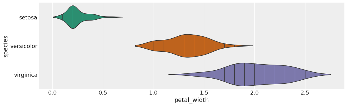
# @title species vs petal_width

from matplotlib import pyplot as plt
import seaborn as sns
figsize = (12, 1.2 * len(iris['species'].unique()))
plt.figure(figsize=figsize)
sns.violinplot(iris, x='petal_width', y='species', inner='stick', palette='Dark2')
sns.despine(top=True, right=True, bottom=True, left=True)

<ipython-input-6-7a5e472054ba>:7: FutureWarning: 

Passing `palette` without assigning `hue` is deprecated and will be removed in v0.14.0. Assign the `y` variable to `hue` and set `legend=False` for the same effect.

  sns.violinplot(iris, x='petal_width', y='species', inner='stick', palette='Dark2')

Recipe 1: Dealing with correlated data#

corr = iris[iris['species'] != 'virginica'].corr()
mask = np.tri(*corr.shape).T
g = sns.heatmap(corr.abs(), mask=mask, annot=True, cmap='viridis')
g.set_xticklabels(g.get_yticklabels(), rotation = 90, fontsize = 14)
g.set_yticklabels(g.get_yticklabels(), rotation = 0, fontsize = 14)

<ipython-input-7-c7a84d82f61e>:1: FutureWarning: The default value of numeric_only in DataFrame.corr is deprecated. In a future version, it will default to False. Select only valid columns or specify the value of numeric_only to silence this warning.
  corr = iris[iris['species'] != 'virginica'].corr()

[Text(0, 0.5, 'sepal_length'),
 Text(0, 1.5, 'sepal_width'),
 Text(0, 2.5, 'petal_length'),
 Text(0, 3.5, 'petal_width')]

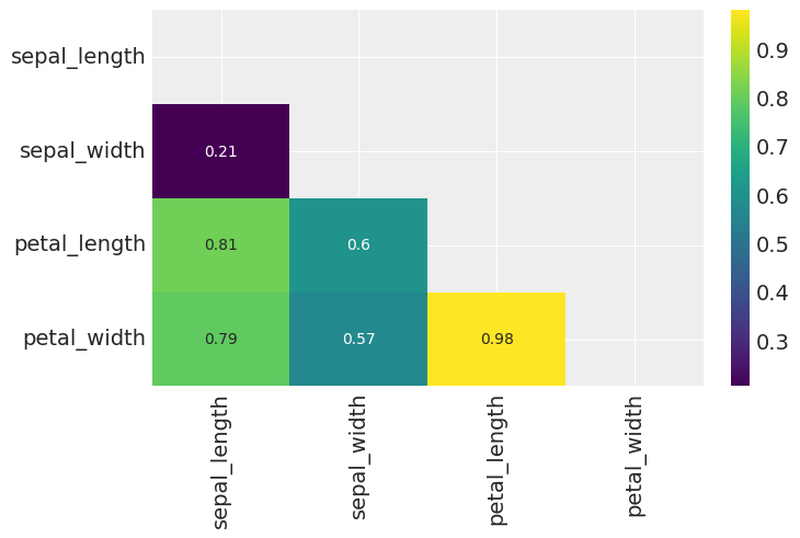
Notes

(i) Correlated data has typically less power to restrict the model; correlated variables translate into wider combinations of coefficients that are able to explain the data.

(ii) One solution when dealing with highly correlated variables is to remove one (or more than one) correlated variable.

(iii) Another option is scaling all non-binary variables to have a mean of 0, and then using (see logistic regression model parameters):

\(\beta \sim StudentT(0,\nu,sd)\) \(sd\) should be chosen to weekly inform us about the expected value for the scale. The normality parameter \(\nu\) is typically chosen to be in the range (3,7). This prior is saying that in general we expect the coefficienct to be small, but we use wide tails because occasionally we will find some larger coefficients.

Recipe 2: Dealing with correlated data#

df = iris.query("species == ('setosa', 'versicolor')")
df = df[45:]   # let's select two unbalanced classes
y_unb = pd.Categorical(df['species']).codes
x_n = ['sepal_length', 'sepal_width']
x_unb = df[x_n].values

print(y_unb) #this is why is unbalanced

[0 0 0 0 0 1 1 1 1 1 1 1 1 1 1 1 1 1 1 1 1 1 1 1 1 1 1 1 1 1 1 1 1 1 1 1 1
 1 1 1 1 1 1 1 1 1 1 1 1 1 1 1 1 1 1]

Doing the usual thing: build the logistic regression…

with pm.Model() as model_unb:
    α = pm.Normal('α', mu=0, sigma=10)
    β = pm.Normal('β', mu=0, sigma=2, shape=len(x_n))

    μ = α + pm.math.dot(x_unb, β)
    θ = 1 / (1 + pm.math.exp(-μ))
    bd = pm.Deterministic('bd', -α/β[1] - β[0]/β[1] * x_unb[:,0])

    yl = pm.Bernoulli('yl', p=θ, observed=y_unb)

    trace_unb = pm.sample(1000, target_accept=0.95)

100.00% [2000/2000 00:32<00:00 Sampling chain 0, 0 divergences]

100.00% [2000/2000 00:15<00:00 Sampling chain 1, 0 divergences]

idx = np.argsort(x_unb[:,0])

bd = trace_unb.posterior['bd'].mean(axis=0).mean(axis=0)[idx]

plt.scatter(x_unb[:,0], x_unb[:,1], c= [f'C{x}' for x in y_unb])
plt.plot(x_unb[:,0][idx], bd, color='k')

az.plot_hdi(x_unb[:,0], trace_unb.posterior['bd'], color='k')

plt.xlabel(x_n[0])
plt.ylabel(x_n[1])

Text(0, 0.5, 'sepal_width')

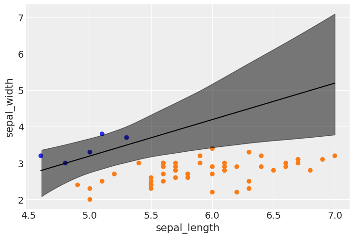
Notes

(i) In case of an unbalanced dataset, logistic regression can run into some trouble: the boundary cannot be determined as accurately as when the dataset is more balanced.

(ii) The decision boundary is “shifted” towards the less abundant class, and the uncertainty band is larger.

(iii) It is always good to have a balanced dataset. If you do have unbalanced data though, you should be careful when you interpret results: check the uncertainty of the model, and run some posterior predictive checks for consistency. Another option is to input more prior information if available and/or run an alternative model.

Generalization to multiple classes: Softmax Regression#

Notes

In order to generalize to mutliple classes, two modifications are needed:

(i) We use a softmax (see also Boltzmann distribution in physics), which is defined as:

\(softmax_{i}(\mu)= \frac{exp(\mu_{i})}{\sum_{k}exp(\mu_{k})}\)

(ii) We then replace the Bernoulli distribution with the categorical distribution. As the Bernoulli (single coin flip) is a special case of a Binomial (n coin flips), the categorical (single roll of a die) is a special case of the multinomial distribution (n rolls of a die).

iris.columns[:-1]

Index(['sepal_length', 'sepal_width', 'petal_length', 'petal_width'], dtype='object')

iris = sns.load_dataset('iris')
y_s = pd.Categorical(iris['species']).codes
x_n = iris.columns[:-1]
x_s = iris[x_n].values

x_s = (x_s - x_s.mean(axis=0)) / x_s.std(axis=0)

print(np.shape(x_s))
print(np.shape(y_s))
#print(x_n)
#print(iris)

(150, 4)
(150,)

with pm.Model() as model_s:
    α = pm.Normal('α', mu=0, sigma=5, shape=3)
    β = pm.Normal('β', mu=0, sigma=5, shape=(4,3))
    μ = pm.Deterministic('μ', α + pm.math.dot(x_s, β))
    θ = pm.math.softmax(μ, axis = 1)
    yl = pm.Categorical('yl', p=θ, observed=y_s)
    idata_s = pm.sample(2000, target_accept=.95)

100.00% [3000/3000 01:13<00:00 Sampling chain 0, 0 divergences]

100.00% [3000/3000 01:16<00:00 Sampling chain 1, 0 divergences]

Note that you need to call .eval() on Theano tensors to convert them to NumPy arrays before passing them to the softmax function.

data_pred = idata_s.posterior['μ'].mean(axis=0).mean(axis=0).values
print(np.shape(data_pred))
print(np.shape(y_s))

(150, 3)
(150,)

y_pred = [np.exp(point)/np.sum(np.exp(point), axis=0)
          for point in data_pred]

res_t = np.sum(y_s == np.argmax(y_pred, axis=1)) / len(y_s)
print("accuracy is: {:1.3f}".format(res_t))

accuracy is: 0.980

az.summary(idata_s).head(15)

/usr/local/lib/python3.10/dist-packages/arviz/utils.py:184: NumbaDeprecationWarning: The 'nopython' keyword argument was not supplied to the 'numba.jit' decorator. The implicit default value for this argument is currently False, but it will be changed to True in Numba 0.59.0. See https://numba.readthedocs.io/en/stable/reference/deprecation.html#deprecation-of-object-mode-fall-back-behaviour-when-using-jit for details.
  numba_fn = numba.jit(**self.kwargs)(self.function)

	mean	sd	hdi_3%	hdi_97%	mcse_mean	mcse_sd	ess_bulk	ess_tail	r_hat
α[0]	-1.128	3.766	-7.880	6.266	0.066	0.054	3236.0	2625.0	1.0
α[1]	5.855	3.194	0.224	12.107	0.060	0.043	2830.0	2885.0	1.0
α[2]	-4.826	3.432	-11.594	1.316	0.061	0.045	3133.0	2971.0	1.0
β[0, 0]	-2.461	4.161	-10.526	5.205	0.067	0.059	3794.0	3053.0	1.0
β[0, 1]	1.970	3.316	-4.186	8.424	0.068	0.050	2369.0	2622.0	1.0
β[0, 2]	0.606	3.332	-5.372	7.274	0.069	0.052	2312.0	2244.0	1.0
β[1, 0]	3.258	3.395	-2.710	9.906	0.066	0.048	2678.0	2749.0	1.0
β[1, 1]	-0.864	3.025	-6.356	5.093	0.064	0.046	2235.0	2242.0	1.0
β[1, 2]	-2.268	3.050	-8.011	3.336	0.065	0.046	2227.0	2475.0	1.0
β[2, 0]	-6.319	4.300	-14.562	1.564	0.071	0.054	3708.0	2755.0	1.0
β[2, 1]	-1.555	3.654	-8.427	5.317	0.062	0.054	3526.0	3002.0	1.0
β[2, 2]	7.660	3.772	0.598	14.655	0.061	0.044	3796.0	3133.0	1.0
β[3, 0]	-5.829	4.248	-14.152	2.004	0.074	0.055	3292.0	3136.0	1.0
β[3, 1]	-0.888	3.486	-7.276	5.645	0.068	0.049	2625.0	3028.0	1.0
β[3, 2]	6.956	3.616	0.164	13.683	0.070	0.051	2697.0	2893.0	1.0

Notes

(i) 98% is the accuracy on our data; a true test to evaluate the performance of our model will be to check it on data not used to fit the model

(ii) You can check that we obtained a wide posterior. This is a result of the fact softmax normalizes probability to 1. Therefore, when we used priors on the parameters of 4 species, in reality we can “eliminate” one species” from the problem, in that one of them can be calculated from the other 3 once we know their probabilities (again, they have to sum up to 1!)

(iii) Below is a suggested solution, that does fix the extra parameters to some value, e.g., zero

with pm.Model() as model_sf:
    α = pm.Normal('α', mu=0, sigma=2, shape=2)
    β = pm.Normal('β', mu=0, sigma=2, shape=(4,2))
    α_f = pm.math.concatenate([[0] ,α])
    β_f = pm.math.concatenate([np.zeros((4,1)) , β], axis=1)
    μ = pm.Deterministic('μ', α_f + pm.math.dot(x_s, β_f))
    θ = pm.math.softmax(μ, axis = 1)
    yl = pm.Categorical('yl', p=θ, observed=y_s)
    idata_sf = pm.sample(2000, target_accept=.92)

100.00% [3000/3000 00:31<00:00 Sampling chain 0, 0 divergences]

100.00% [3000/3000 00:33<00:00 Sampling chain 1, 0 divergences]

data_pred_sf = idata_sf.posterior['μ'].mean(axis=0).mean(axis=0).values

y_pred_sf = [np.exp(point)/np.sum(np.exp(point), axis=0)
          for point in data_pred_sf]

res_sf = np.sum(y_s == np.argmax(y_pred_sf, axis=1)) / len(y_s)
print("accuracy is: {:1.3f}".format(res_sf))

accuracy is: 0.973

mu_pred = idata_sf.posterior['μ'].mean(axis=0)
print(np.shape(mu_pred), type(mu_pred))

(2000, 150, 3) <class 'xarray.core.dataarray.DataArray'>

import xarray as xr

def softmax(x):
    e_x = np.exp(x)
    return e_x.values / np.sum(e_x, axis = 2, keepdims=True).values

res_sm= softmax(mu_pred)
print(np.shape(res_sm))

(2000, 150, 3)

# Average probabilities for prediction
mean_probabilities = np.mean(res_sm, axis=0)

# Uncertainty estimation
lower_bound = np.percentile(res_sm, 2.5, axis=0)
upper_bound = np.percentile(res_sm, 97.5, axis=0)

# class_assignment
class_prediction = np.argmax(y_pred_sf, axis=1)

print(np.shape(class_prediction),np.shape(mean_probabilities),np.shape(lower_bound))

(150,) (150, 3) (150, 3)

print("\n" + "=" * 39)
print("DATA:")
print("=" * 39)

print("class, probabilities, ranges(94%HDI):")
for count, (g, h, i, j, k) in enumerate(zip(y_s, class_prediction, mean_probabilities, lower_bound, upper_bound)):
    print(f"data point: {count}, ground-truth: {g}, class: {h}")
    for l in range(3):
        print(f"    idx: {l}, mean prob. {i[l]:.4f}, 94% HDI: [{j[l]:.4f},{k[l]:.4f}]")
    if count >= 5:
      break
print("=" * 39)

=======================================
DATA:
=======================================
class, probabilities, ranges(94%HDI):
data point: 0, ground-truth: 0, class: 0
    idx: 0, mean prob. 0.9905, 94% HDI: [0.9698,0.9991]
    idx: 1, mean prob. 0.0095, 94% HDI: [0.0009,0.0302]
    idx: 2, mean prob. 0.0000, 94% HDI: [0.0000,0.0000]
data point: 1, ground-truth: 0, class: 0
    idx: 0, mean prob. 0.9579, 94% HDI: [0.8851,0.9927]
    idx: 1, mean prob. 0.0421, 94% HDI: [0.0073,0.1149]
    idx: 2, mean prob. 0.0000, 94% HDI: [0.0000,0.0000]
data point: 2, ground-truth: 0, class: 0
    idx: 0, mean prob. 0.9893, 94% HDI: [0.9682,0.9987]
    idx: 1, mean prob. 0.0107, 94% HDI: [0.0013,0.0318]
    idx: 2, mean prob. 0.0000, 94% HDI: [0.0000,0.0000]
data point: 3, ground-truth: 0, class: 0
    idx: 0, mean prob. 0.9845, 94% HDI: [0.9522,0.9981]
    idx: 1, mean prob. 0.0155, 94% HDI: [0.0019,0.0478]
    idx: 2, mean prob. 0.0000, 94% HDI: [0.0000,0.0000]
data point: 4, ground-truth: 0, class: 0
    idx: 0, mean prob. 0.9948, 94% HDI: [0.9820,0.9996]
    idx: 1, mean prob. 0.0052, 94% HDI: [0.0004,0.0180]
    idx: 2, mean prob. 0.0000, 94% HDI: [0.0000,0.0000]
data point: 5, ground-truth: 0, class: 0
    idx: 0, mean prob. 0.9917, 94% HDI: [0.9660,0.9996]
    idx: 1, mean prob. 0.0083, 94% HDI: [0.0004,0.0340]
    idx: 2, mean prob. 0.0000, 94% HDI: [0.0000,0.0000]
=======================================

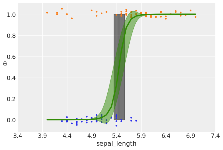
Final remarks: Robust Logistic Regression (extra, for the curious…)#

Let’s take the dataset for the species setosa and versicolor only. Let’s complicate the problem by assuming the presence of unusual seros and/or ones in our dataset.

iris = sns.load_dataset("iris")
df = iris.query("species == ('setosa', 'versicolor')")
y_0 = pd.Categorical(df['species']).codes
x_n = 'sepal_length'
x_0 = df[x_n].values
y_0 = np.concatenate((y_0, np.ones(6, dtype=int)))
x_0 = np.concatenate((x_0, [4.2, 4.5, 4.0, 4.3, 4.2, 4.4]))
x_c = x_0 - x_0.mean()
plt.plot(x_c, y_0, 'o', color='k');
plt.xlabel(x_n)

Text(0.5, 0, 'sepal_length')

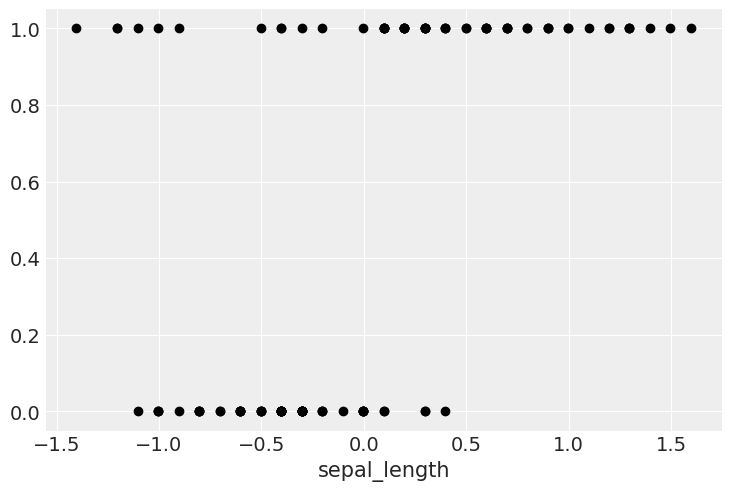
We have some versicolor (category 1) with some unusually short sepal_length…

We can fix this with a mixture model. We say that the outpu variable comes with \(\pi\) probability of random guessing (0.5 chance for category 1 to be indeed 1), and with 1-\(\pi\) probability from a logistic regression model:

\(p= \pi \ 0.5 + (1-\pi) \ logistic(\alpha+X\beta)\)

Notice that when \(\pi=1\), we get \(p=0.5\) (random guess), whereas when \(\pi=0\) we get the logistic regression.

This model can be implemented with a slight modification of what we saw before.

N.B. \(\pi\) is a new variable in our model

with pm.Model() as model_rlg:
    α = pm.Normal('α', mu=0, sigma=10)
    β = pm.Normal('β', mu=0, sigma=10)

    μ = α + x_c *  β
    θ = pm.Deterministic('θ', pm.math.sigmoid(μ))
    bd = pm.Deterministic('bd', -α/β)

    π = pm.Beta('π', 1., 1.)
    p = π * 0.5 + (1 - π) * θ

    yl = pm.Bernoulli('yl', p=p, observed=y_0)

    idata_rlg = pm.sample(2000, target_accept=0.95,  tune = 2000, return_inferencedata=True)

100.00% [4000/4000 00:08<00:00 Sampling chain 0, 0 divergences]

100.00% [4000/4000 00:08<00:00 Sampling chain 1, 1 divergences]

theta = idata_rlg.posterior['θ'].mean(axis=0).mean(axis=0)
idx = np.argsort(x_c)

np.random.seed(123)

plt.plot(x_c[idx], theta[idx], color='C2', lw=3)

plt.vlines(idata_rlg.posterior['bd'].mean(), 0, 1, color='k')

bd_hpd = az.hdi(idata_rlg.posterior['bd'])

plt.fill_betweenx([0, 1], bd_hpd.bd[0].values, bd_hpd.bd[1].values, color='k', alpha=0.5)

plt.scatter(x_c, np.random.normal(y_0, 0.02),
            marker='.', color=[f'C{x}' for x in y_0])

az.plot_hdi(x_c, idata_rlg.posterior['θ'], color='C2')  #green band

plt.xlabel(x_n)
plt.ylabel('θ', rotation=0)
# use original scale for xticks
locs, _ = plt.xticks()
plt.xticks(locs, np.round(locs + x_0.mean(), 1))

([<matplotlib.axis.XTick at 0x7d1db3434c10>,
  <matplotlib.axis.XTick at 0x7d1db3437be0>,
  <matplotlib.axis.XTick at 0x7d1e1727a2c0>,
  <matplotlib.axis.XTick at 0x7d1db3d28f40>,
  <matplotlib.axis.XTick at 0x7d1dbf50bdf0>,
  <matplotlib.axis.XTick at 0x7d1db3b2afe0>,
  <matplotlib.axis.XTick at 0x7d1db3d3cac0>,
  <matplotlib.axis.XTick at 0x7d1db3b988b0>,
  <matplotlib.axis.XTick at 0x7d1db3b993f0>],
 [Text(-2.0, 0, '3.4'),
  Text(-1.5, 0, '3.9'),
  Text(-1.0, 0, '4.4'),
  Text(-0.5, 0, '4.9'),
  Text(0.0, 0, '5.4'),
  Text(0.5, 0, '5.9'),
  Text(1.0, 0, '6.4'),
  Text(1.5, 0, '6.9'),
  Text(2.0, 0, '7.4')])

Bayesian Reasoning in Data Science (DATA 644)

Generalization to Bayesian Softmax Regression

Contents

Generalization to Bayesian Softmax Regression#

Recipe 1: Dealing with correlated data#

Recipe 2: Dealing with correlated data#

Generalization to multiple classes: Softmax Regression#

Final remarks: Robust Logistic Regression (extra, for the curious…)#