Gaussian Processes

%pip install pymc pytensor

Requirement already satisfied: pymc in /usr/local/lib/python3.10/dist-packages (5.10.4)
Requirement already satisfied: pytensor in /usr/local/lib/python3.10/dist-packages (2.18.6)
Requirement already satisfied: arviz>=0.13.0 in /usr/local/lib/python3.10/dist-packages (from pymc) (0.15.1)
Requirement already satisfied: cachetools>=4.2.1 in /usr/local/lib/python3.10/dist-packages (from pymc) (5.3.3)
Requirement already satisfied: cloudpickle in /usr/local/lib/python3.10/dist-packages (from pymc) (2.2.1)
Requirement already satisfied: fastprogress>=0.2.0 in /usr/local/lib/python3.10/dist-packages (from pymc) (1.0.3)
Requirement already satisfied: numpy>=1.15.0 in /usr/local/lib/python3.10/dist-packages (from pymc) (1.25.2)
Requirement already satisfied: pandas>=0.24.0 in /usr/local/lib/python3.10/dist-packages (from pymc) (1.5.3)
Requirement already satisfied: scipy>=1.4.1 in /usr/local/lib/python3.10/dist-packages (from pymc) (1.11.4)
Requirement already satisfied: typing-extensions>=3.7.4 in /usr/local/lib/python3.10/dist-packages (from pymc) (4.10.0)
Requirement already satisfied: setuptools>=48.0.0 in /usr/local/lib/python3.10/dist-packages (from pytensor) (67.7.2)
Requirement already satisfied: filelock in /usr/local/lib/python3.10/dist-packages (from pytensor) (3.13.1)
Requirement already satisfied: etuples in /usr/local/lib/python3.10/dist-packages (from pytensor) (0.3.9)
Requirement already satisfied: logical-unification in /usr/local/lib/python3.10/dist-packages (from pytensor) (0.4.6)
Requirement already satisfied: miniKanren in /usr/local/lib/python3.10/dist-packages (from pytensor) (1.0.3)
Requirement already satisfied: cons in /usr/local/lib/python3.10/dist-packages (from pytensor) (0.4.6)
Requirement already satisfied: matplotlib>=3.2 in /usr/local/lib/python3.10/dist-packages (from arviz>=0.13.0->pymc) (3.7.1)
Requirement already satisfied: packaging in /usr/local/lib/python3.10/dist-packages (from arviz>=0.13.0->pymc) (24.0)
Requirement already satisfied: xarray>=0.21.0 in /usr/local/lib/python3.10/dist-packages (from arviz>=0.13.0->pymc) (2023.7.0)
Requirement already satisfied: h5netcdf>=1.0.2 in /usr/local/lib/python3.10/dist-packages (from arviz>=0.13.0->pymc) (1.3.0)
Requirement already satisfied: xarray-einstats>=0.3 in /usr/local/lib/python3.10/dist-packages (from arviz>=0.13.0->pymc) (0.7.0)
Requirement already satisfied: python-dateutil>=2.8.1 in /usr/local/lib/python3.10/dist-packages (from pandas>=0.24.0->pymc) (2.8.2)
Requirement already satisfied: pytz>=2020.1 in /usr/local/lib/python3.10/dist-packages (from pandas>=0.24.0->pymc) (2023.4)
Requirement already satisfied: toolz in /usr/local/lib/python3.10/dist-packages (from logical-unification->pytensor) (0.12.1)
Requirement already satisfied: multipledispatch in /usr/local/lib/python3.10/dist-packages (from logical-unification->pytensor) (1.0.0)
Requirement already satisfied: h5py in /usr/local/lib/python3.10/dist-packages (from h5netcdf>=1.0.2->arviz>=0.13.0->pymc) (3.9.0)
Requirement already satisfied: contourpy>=1.0.1 in /usr/local/lib/python3.10/dist-packages (from matplotlib>=3.2->arviz>=0.13.0->pymc) (1.2.0)
Requirement already satisfied: cycler>=0.10 in /usr/local/lib/python3.10/dist-packages (from matplotlib>=3.2->arviz>=0.13.0->pymc) (0.12.1)
Requirement already satisfied: fonttools>=4.22.0 in /usr/local/lib/python3.10/dist-packages (from matplotlib>=3.2->arviz>=0.13.0->pymc) (4.50.0)
Requirement already satisfied: kiwisolver>=1.0.1 in /usr/local/lib/python3.10/dist-packages (from matplotlib>=3.2->arviz>=0.13.0->pymc) (1.4.5)
Requirement already satisfied: pillow>=6.2.0 in /usr/local/lib/python3.10/dist-packages (from matplotlib>=3.2->arviz>=0.13.0->pymc) (9.4.0)
Requirement already satisfied: pyparsing>=2.3.1 in /usr/local/lib/python3.10/dist-packages (from matplotlib>=3.2->arviz>=0.13.0->pymc) (3.1.2)
Requirement already satisfied: six>=1.5 in /usr/local/lib/python3.10/dist-packages (from python-dateutil>=2.8.1->pandas>=0.24.0->pymc) (1.16.0)

import numpy as np
import matplotlib.pyplot as plt
from scipy import stats
import pymc as pm

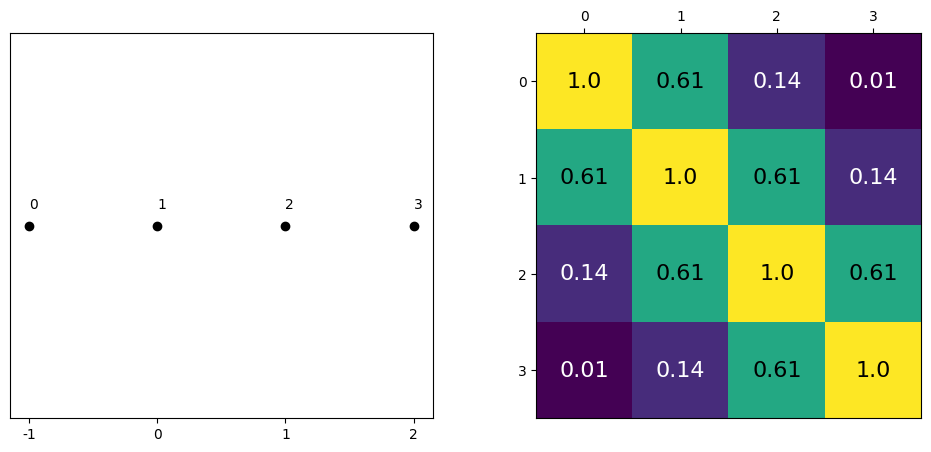
Covariance Functions and Kernel

def exp_quad_kernel(x,knots,l=1):
  return np.array([np.exp(-(x-k)**2/(2*l**2)) for k in knots])

data = np.array([-1,0,1,2])
#data = np.array([-1,0])
cov = exp_quad_kernel(data,data,1)

print(cov)

[[1.         0.60653066 0.13533528 0.011109  ]
 [0.60653066 1.         0.60653066 0.13533528]
 [0.13533528 0.60653066 1.         0.60653066]
 [0.011109   0.13533528 0.60653066 1.        ]]

_, ax=plt.subplots(1,2,figsize=(12,5))

ax[0].plot(data, np.zeros_like(data),'ko')
ax[0].set_yticks([])

for idx,i in enumerate(data):
  ax[0].text(i,0+0.005, idx)
ax[0].set_xticks(data)
ax[0].set_xticklabels(np.round(data,2))

ax[1].grid(False)
im = ax[1].imshow(cov)
colors=['w','k']

for i in range(len(cov)):
  for j in range(len(cov)):
    ax[1].text(i,j, round(cov[i,j],2), color=colors[int(im.norm(cov[i,j])>0.5)], ha = 'center', va='center', fontdict={'size':16})

ax[1].set_xticks(range(len(data)))
ax[1].set_yticks(range(len(data)))
ax[1].xaxis.tick_top()

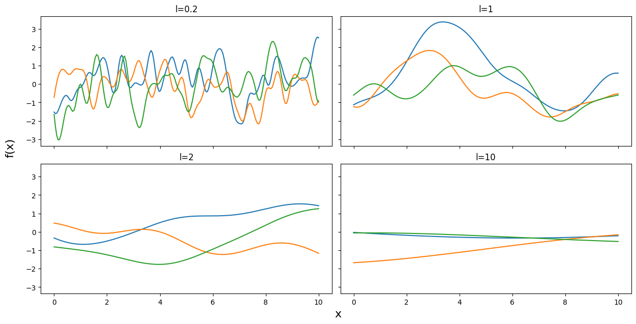
np.random.seed(24)
test_points = np.linspace(0,10,200)
fig, ax = plt.subplots(2,2,figsize=(12,6),sharex=True,sharey=True,constrained_layout=True)
ax = np.ravel(ax)
for idx, l in enumerate((0.2,1,2,10)):
  cov = exp_quad_kernel(test_points, test_points, l)
  ax[idx].plot(test_points, stats.multivariate_normal.rvs(cov=cov,size=3).T)
  ax[idx].set_title(f'l={l}')

fig.text(0.51,-0.03,'x', fontsize=16)
fig.text(-0.03,0.5,'f(x)', fontsize=16, rotation=90)

Text(-0.03, 0.5, 'f(x)')

Gaussian Processes: Implementation

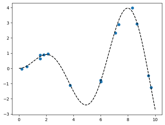
np.random.seed(42)

x = np.random.uniform(0,10,size=15)

scale = 0.50
y = np.random.normal(scale*x*np.sin(x), 0.1)

plt.plot(x,y,'o')

true_x = np.linspace(0,10,200)
true_y = scale*true_x*np.sin(true_x)
plt.plot(true_x,true_y, 'k--')

[<matplotlib.lines.Line2D at 0x7e097098ec50>]

X = x[:,None]

with pm.Model() as model_reg:
  #hyperprior for lengthscale kernel parameter
  l = pm.Gamma('l',2,0.5)
  #instantiate a covariance function
  cov = pm.gp.cov.ExpQuad(1,ls=l)
  #mean = pm.gp.mean.Constant(c=0)
  #instantiate a GP prior
  gp = pm.gp.Marginal(cov_func=cov)#mean_func=mean,
  #prior
  eps = pm.HalfNormal('eps',25)
  #likelihood
  y_pred = gp.marginal_likelihood('y_pred',X=X, y=y, noise=eps)
  trace_reg = pm.sample(2000, return_inferencedata=True, target_accept=0.95)

/usr/local/lib/python3.10/dist-packages/pymc/gp/gp.py:56: FutureWarning: The 'noise' parameter has been been changed to 'sigma' in order to standardize the GP API and will be deprecated in future releases.
  warnings.warn(_noise_deprecation_warning, FutureWarning)

100.00% [3000/3000 00:19<00:00 Sampling chain 0, 0 divergences]

100.00% [3000/3000 00:23<00:00 Sampling chain 1, 0 divergences]

import arviz as az
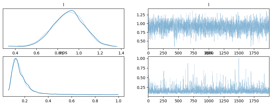
az.plot_trace(trace_reg)

/usr/local/lib/python3.10/dist-packages/arviz/utils.py:184: NumbaDeprecationWarning: The 'nopython' keyword argument was not supplied to the 'numba.jit' decorator. The implicit default value for this argument is currently False, but it will be changed to True in Numba 0.59.0. See https://numba.readthedocs.io/en/stable/reference/deprecation.html#deprecation-of-object-mode-fall-back-behaviour-when-using-jit for details.
  numba_fn = numba.jit(**self.kwargs)(self.function)

array([[<Axes: title={'center': 'l'}>, <Axes: title={'center': 'l'}>],
       [<Axes: title={'center': 'eps'}>, <Axes: title={'center': 'eps'}>]],
      dtype=object)

X_new = np.linspace(np.floor(x.min()), np.ceil(x.max()), 100)[:,None]

with model_reg:
    #del marginal_gp_model.named_vars['f_pred']
    #marginal_gp_model.vars.remove(f_pred)
    f_pred = gp.conditional('f_pred', X_new)

with model_reg:
    pred_samples = pm.sample_posterior_predictive(trace_reg, var_names=['f_pred'])

100.00% [4000/4000 00:53<00:00]

pred_samples

arviz.InferenceData

• posterior_predictive

  <xarray.Dataset>
  Dimensions:       (chain: 2, draw: 2000, f_pred_dim_2: 100)
  Coordinates:
    * chain         (chain) int64 0 1
    * draw          (draw) int64 0 1 2 3 4 5 6 ... 1994 1995 1996 1997 1998 1999
    * f_pred_dim_2  (f_pred_dim_2) int64 0 1 2 3 4 5 6 7 ... 93 94 95 96 97 98 99
  Data variables:
      f_pred        (chain, draw, f_pred_dim_2) float64 0.0928 0.04929 ... -2.191
  Attributes:
      created_at:                 2024-03-26T01:56:59.862834
      arviz_version:              0.15.1
      inference_library:          pymc
      inference_library_version:  5.10.4

  xarray.Dataset

  • Dimensions:
    • chain: 2
    • draw: 2000
    • f_pred_dim_2: 100
  • Coordinates: (3)
    • chain
      (chain)
      int64
      0 1

      array([0, 1])

    • draw
      (draw)
      int64
      0 1 2 3 4 ... 1996 1997 1998 1999

      array([   0,    1,    2, ..., 1997, 1998, 1999])

    • f_pred_dim_2
      (f_pred_dim_2)
      int64
      0 1 2 3 4 5 6 ... 94 95 96 97 98 99

      array([ 0,  1,  2,  3,  4,  5,  6,  7,  8,  9, 10, 11, 12, 13, 14, 15, 16, 17,
             18, 19, 20, 21, 22, 23, 24, 25, 26, 27, 28, 29, 30, 31, 32, 33, 34, 35,
             36, 37, 38, 39, 40, 41, 42, 43, 44, 45, 46, 47, 48, 49, 50, 51, 52, 53,
             54, 55, 56, 57, 58, 59, 60, 61, 62, 63, 64, 65, 66, 67, 68, 69, 70, 71,
             72, 73, 74, 75, 76, 77, 78, 79, 80, 81, 82, 83, 84, 85, 86, 87, 88, 89,
             90, 91, 92, 93, 94, 95, 96, 97, 98, 99])

  • Data variables: (1)
    • f_pred
      (chain, draw, f_pred_dim_2)
      float64
      0.0928 0.04929 ... -1.908 -2.191

      array([[[ 9.27993240e-02,  4.92906221e-02,  1.09413426e-02, ...,
               -1.26525887e+00, -1.44613655e+00, -1.58752713e+00],
              [-8.36048697e-03,  1.67208930e-02,  5.66319096e-02, ...,
               -1.03970070e+00, -1.15337437e+00, -1.21319211e+00],
              [-3.58550513e-02, -2.23645317e-02,  4.91028470e-03, ...,
               -1.37112971e+00, -1.49412783e+00, -1.56061126e+00],
              ...,
              [ 3.57315098e-02, -2.77640983e-03, -2.90906480e-02, ...,
               -1.19841712e+00, -1.37517217e+00, -1.48323916e+00],
              [ 2.25621379e-01,  1.94148294e-01,  1.66403958e-01, ...,
               -1.29723467e+00, -1.47140633e+00, -1.60085940e+00],
              [ 7.76021479e-02,  4.82590946e-02,  2.25220782e-02, ...,
               -1.40292567e+00, -1.56997179e+00, -1.68859158e+00]],
      
             [[-2.98168881e-01, -2.71137349e-01, -2.35434093e-01, ...,
               -1.26324350e+00, -1.44859271e+00, -1.58839589e+00],
              [ 2.65615457e-02, -3.73443992e-02, -8.20272969e-02, ...,
               -1.20353198e+00, -1.35934550e+00, -1.46372070e+00],
              [ 1.47851200e-01,  1.32791626e-01,  1.21124073e-01, ...,
               -1.47532664e+00, -1.68233182e+00, -1.81958248e+00],
              ...,
              [ 1.43914741e-01,  8.54822438e-02,  4.40057986e-02, ...,
               -1.28217775e+00, -1.47958488e+00, -1.63357374e+00],
              [-3.56892471e-01, -3.03687926e-01, -2.34737874e-01, ...,
               -1.25261092e+00, -1.44772836e+00, -1.60892327e+00],
              [ 1.61214329e-03, -1.17824401e-02, -8.42623526e-03, ...,
               -1.59229325e+00, -1.90814886e+00, -2.19113669e+00]]])

  • Indexes: (3)
    • chain
      PandasIndex

      PandasIndex(Int64Index([0, 1], dtype='int64', name='chain'))

    • draw
      PandasIndex

      PandasIndex(Int64Index([   0,    1,    2,    3,    4,    5,    6,    7,    8,    9,
                  ...
                  1990, 1991, 1992, 1993, 1994, 1995, 1996, 1997, 1998, 1999],
                 dtype='int64', name='draw', length=2000))

    • f_pred_dim_2
      PandasIndex

      PandasIndex(Int64Index([ 0,  1,  2,  3,  4,  5,  6,  7,  8,  9, 10, 11, 12, 13, 14, 15, 16,
                  17, 18, 19, 20, 21, 22, 23, 24, 25, 26, 27, 28, 29, 30, 31, 32, 33,
                  34, 35, 36, 37, 38, 39, 40, 41, 42, 43, 44, 45, 46, 47, 48, 49, 50,
                  51, 52, 53, 54, 55, 56, 57, 58, 59, 60, 61, 62, 63, 64, 65, 66, 67,
                  68, 69, 70, 71, 72, 73, 74, 75, 76, 77, 78, 79, 80, 81, 82, 83, 84,
                  85, 86, 87, 88, 89, 90, 91, 92, 93, 94, 95, 96, 97, 98, 99],
                 dtype='int64', name='f_pred_dim_2'))

  • Attributes: (4)

    created_at :

    2024-03-26T01:56:59.862834

    arviz_version :

    0.15.1

    inference_library :

    pymc

    inference_library_version :

    5.10.4

  
  
• observed_data

  <xarray.Dataset>
  Dimensions:       (y_pred_dim_0: 15)
  Coordinates:
    * y_pred_dim_0  (y_pred_dim_0) int64 0 1 2 3 4 5 6 7 8 9 10 11 12 13 14
  Data variables:
      y_pred        (y_pred_dim_0) float64 -1.12 -0.4835 2.889 ... 0.9431 0.8937
  Attributes:
      created_at:                 2024-03-26T01:56:59.864786
      arviz_version:              0.15.1
      inference_library:          pymc
      inference_library_version:  5.10.4

  xarray.Dataset

  • Dimensions:
    • y_pred_dim_0: 15
  • Coordinates: (1)
    • y_pred_dim_0
      (y_pred_dim_0)
      int64
      0 1 2 3 4 5 6 7 8 9 10 11 12 13 14

      array([ 0,  1,  2,  3,  4,  5,  6,  7,  8,  9, 10, 11, 12, 13, 14])

  • Data variables: (1)
    • y_pred
      (y_pred_dim_0)
      float64
      -1.12 -0.4835 ... 0.9431 0.8937

      array([-1.12042313, -0.48349416,  2.88908801, -0.77981502,  0.8616938 ,
              0.62753908,  0.1165545 ,  2.91885168, -0.87790937,  2.31966448,
             -0.04191073, -1.25393673,  3.96600733,  0.94310182,  0.8936542 ])

  • Indexes: (1)
    • y_pred_dim_0
      PandasIndex

      PandasIndex(Int64Index([0, 1, 2, 3, 4, 5, 6, 7, 8, 9, 10, 11, 12, 13, 14], dtype='int64', name='y_pred_dim_0'))

  • Attributes: (4)

    created_at :

    2024-03-26T01:56:59.864786

    arviz_version :

    0.15.1

    inference_library :

    pymc

    inference_library_version :

    5.10.4

  
  

print(np.shape(pred_samples.posterior_predictive['f_pred'].mean(axis=0).T))
print(np.shape(X_new))

(100, 2000)
(100, 1)

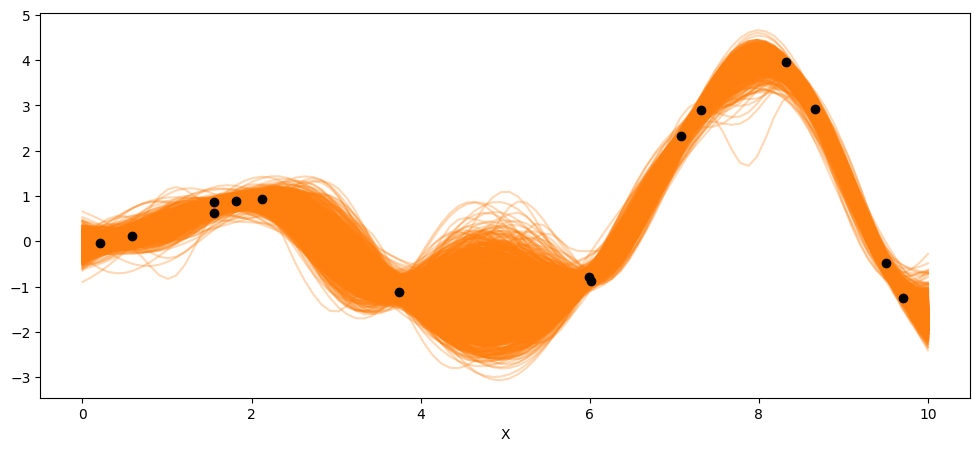
_, ax = plt.subplots(figsize=(12,5))
ax.plot(X_new, pred_samples.posterior_predictive['f_pred'].mean(axis=0).T, 'C1-', alpha=0.3)
ax.plot(X, y, 'ko')
ax.set_xlabel('X')

Text(0.5, 0, 'X')

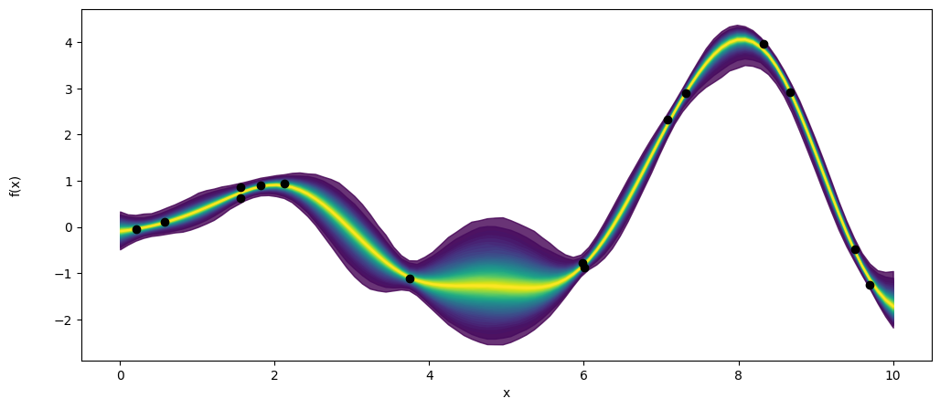
_, ax = plt.subplots(figsize=(12,5))
pm.gp.util.plot_gp_dist(ax, pred_samples.posterior_predictive['f_pred'].mean(axis=0), X_new, palette='viridis',plot_samples=False)

ax.plot(X,y,'ko')
ax.set_xlabel('x')
ax.set_ylabel('f(x)',labelpad=25)

Text(0, 0.5, 'f(x)')

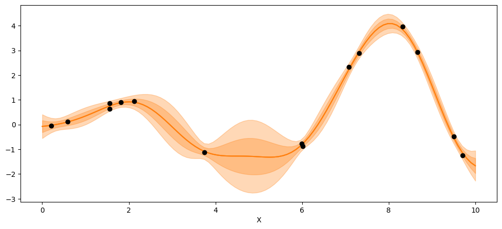
_, ax = plt.subplots(figsize=(12,5))
point = {'l':trace_reg.posterior['l'].mean(), 'eps':trace_reg.posterior['eps'].mean()}

mu, var = gp.predict(X_new, point=point, diag=True, model = model_reg)
sd = var**0.5

ax.plot(X_new,mu,'C1')
ax.fill_between(X_new.flatten(),mu-sd,mu+sd, color="C1",alpha=0.3)

ax.plot(X_new,mu,'C1')
ax.fill_between(X_new.flatten(),mu-2*sd,mu+2*sd, color="C1",alpha=0.3)

ax.plot(X,y,'ko')
ax.set_xlabel('X')

Text(0.5, 0, 'X')

Real-world example: Spawning Salmon

credits: https://github.com/fonnesbeck/gp_tutorial_pydata

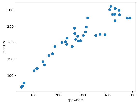
The plot below shows the relationship between the number of spawning salmon in a particular stream and the number of fry that are recruited into the population in the spring.

Biological knowledge suggests this relationship is not linear and we would like to model it.

import requests
import pandas as pd
import io

target_url = 'https://raw.githubusercontent.com/cfteach/brds/main/datasets/salmon.txt'
download = requests.get(target_url).content

salmon_data = pd.read_table(io.StringIO(download.decode('utf-8')), sep='\s+', index_col=0)
salmon_data.plot.scatter(x='spawners', y='recruits', s=50);

#we have prior knowledge about fish population growth, and we can include a linear mean function as a prior

with pm.Model() as salmon_model:

    # Lengthscale
    ρ = pm.HalfCauchy('ρ', 1)
    η = pm.HalfCauchy('η', 1)
    #η=1

    M = pm.gp.mean.Linear(coeffs=(salmon_data.recruits/salmon_data.spawners).mean())
    K = (η**2) * pm.gp.cov.ExpQuad(1, ρ)

with salmon_model:

    σ = pm.HalfCauchy('σ', 1)

    recruit_gp = pm.gp.Marginal(mean_func=M, cov_func=K)
    recruit_gp.marginal_likelihood('recruits', X=salmon_data.spawners.values.reshape(-1,1),
                           y=salmon_data.recruits.values, noise=σ)

/usr/local/lib/python3.10/dist-packages/pymc/gp/gp.py:56: FutureWarning: The 'noise' parameter has been been changed to 'sigma' in order to standardize the GP API and will be deprecated in future releases.
  warnings.warn(_noise_deprecation_warning, FutureWarning)

with salmon_model:
    salmon_trace = pm.sample(1000, return_inferencedata=True)

100.00% [2000/2000 00:22<00:00 Sampling chain 0, 0 divergences]

100.00% [2000/2000 00:22<00:00 Sampling chain 1, 0 divergences]

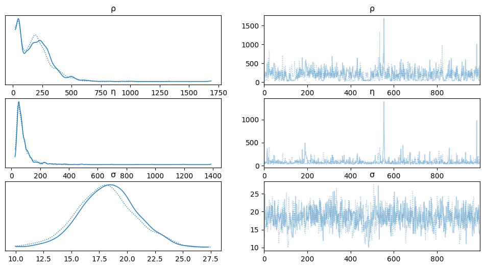
az.plot_trace(salmon_trace, var_names=['ρ','η','σ']) #'η'

array([[<Axes: title={'center': 'ρ'}>, <Axes: title={'center': 'ρ'}>],
       [<Axes: title={'center': 'η'}>, <Axes: title={'center': 'η'}>],
       [<Axes: title={'center': 'σ'}>, <Axes: title={'center': 'σ'}>]],
      dtype=object)

X_pred = np.linspace(0, 500, 100).reshape(-1, 1)

with salmon_model:
    salmon_pred3 = recruit_gp.conditional('salmon_pred3', X_pred)

with salmon_model:
    salmon_samples = pm.sample_posterior_predictive(salmon_trace, var_names=['salmon_pred3'])

100.00% [2000/2000 00:28<00:00]

salmon_data['spawners'].values

array([ 56,  62, 445, 279, 138, 428, 319, 102,  51, 289, 351, 282, 310,
       266, 256, 144, 447, 186, 389, 113, 412, 176, 313, 162, 368,  54,
       214, 429, 115, 407, 265, 301, 234, 229, 270, 478, 419, 490, 430,
       235])

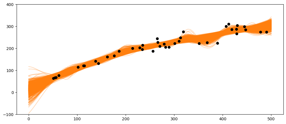
_, ax = plt.subplots(figsize=(12,5))
ax.plot(X_pred, salmon_samples.posterior_predictive['salmon_pred3'].mean(axis=0).T, 'C1-', alpha=0.3)
ax.plot(salmon_data['spawners'].values,salmon_data['recruits'].values, 'ko')
#ax.set_xlabel('X')
ax.set_ylim(-100,400)

(-100.0, 400.0)

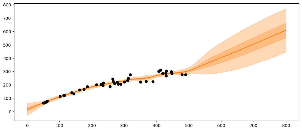
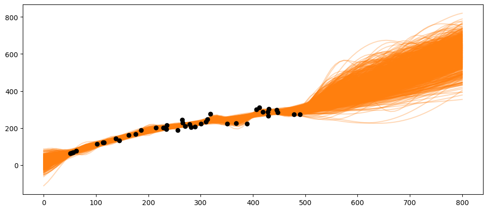
What happens if the population gets very large, e.g., at 600 or 800 spawners?

X_pred = np.linspace(0, 800, 100).reshape(-1, 1)

with salmon_model:
    salmon_pred4 = recruit_gp.conditional('salmon_pred4', X_pred)

with salmon_model:
    salmon_samples = pm.sample_posterior_predictive(salmon_trace, var_names=['salmon_pred4'])

100.00% [2000/2000 00:24<00:00]

_, ax = plt.subplots(figsize=(12,5))
ax.plot(X_pred, salmon_samples.posterior_predictive['salmon_pred4'].mean(axis=0).T, 'C1-', alpha=0.3)
ax.plot(salmon_data['spawners'].values,salmon_data['recruits'].values, 'ko')

[<matplotlib.lines.Line2D at 0x7e0958596380>]

_, ax = plt.subplots(figsize=(12,5))

mu = salmon_samples.posterior_predictive['salmon_pred4'].mean(axis=0).T.mean(axis=1)
sd = salmon_samples.posterior_predictive['salmon_pred4'].std(axis=0).T.mean(axis=1)


ax.plot(X_pred,mu,'C1')
ax.fill_between(X_pred.flatten(),mu-sd,mu+sd, color="C1",alpha=0.3)

ax.plot(X_pred,mu,'C1')
ax.fill_between(X_pred.flatten(),mu-3*sd,mu+3*sd, color="C1",alpha=0.3)


ax.plot(salmon_data['spawners'].values,salmon_data['recruits'].values, 'ko')

[<matplotlib.lines.Line2D at 0x7e0957e302b0>]