Model Comparison#

%pip install pymc pytensor

Requirement already satisfied: pymc in /usr/local/lib/python3.10/dist-packages (5.10.4)
Requirement already satisfied: pytensor in /usr/local/lib/python3.10/dist-packages (2.18.6)
Requirement already satisfied: arviz>=0.13.0 in /usr/local/lib/python3.10/dist-packages (from pymc) (0.15.1)
Requirement already satisfied: cachetools>=4.2.1 in /usr/local/lib/python3.10/dist-packages (from pymc) (5.3.3)
Requirement already satisfied: cloudpickle in /usr/local/lib/python3.10/dist-packages (from pymc) (2.2.1)
Requirement already satisfied: fastprogress>=0.2.0 in /usr/local/lib/python3.10/dist-packages (from pymc) (1.0.3)
Requirement already satisfied: numpy>=1.15.0 in /usr/local/lib/python3.10/dist-packages (from pymc) (1.25.2)
Requirement already satisfied: pandas>=0.24.0 in /usr/local/lib/python3.10/dist-packages (from pymc) (1.5.3)
Requirement already satisfied: scipy>=1.4.1 in /usr/local/lib/python3.10/dist-packages (from pymc) (1.11.4)
Requirement already satisfied: typing-extensions>=3.7.4 in /usr/local/lib/python3.10/dist-packages (from pymc) (4.10.0)
Requirement already satisfied: setuptools>=48.0.0 in /usr/local/lib/python3.10/dist-packages (from pytensor) (67.7.2)
Requirement already satisfied: filelock in /usr/local/lib/python3.10/dist-packages (from pytensor) (3.13.1)
Requirement already satisfied: etuples in /usr/local/lib/python3.10/dist-packages (from pytensor) (0.3.9)
Requirement already satisfied: logical-unification in /usr/local/lib/python3.10/dist-packages (from pytensor) (0.4.6)
Requirement already satisfied: miniKanren in /usr/local/lib/python3.10/dist-packages (from pytensor) (1.0.3)
Requirement already satisfied: cons in /usr/local/lib/python3.10/dist-packages (from pytensor) (0.4.6)
Requirement already satisfied: matplotlib>=3.2 in /usr/local/lib/python3.10/dist-packages (from arviz>=0.13.0->pymc) (3.7.1)
Requirement already satisfied: packaging in /usr/local/lib/python3.10/dist-packages (from arviz>=0.13.0->pymc) (23.2)
Requirement already satisfied: xarray>=0.21.0 in /usr/local/lib/python3.10/dist-packages (from arviz>=0.13.0->pymc) (2023.7.0)
Requirement already satisfied: h5netcdf>=1.0.2 in /usr/local/lib/python3.10/dist-packages (from arviz>=0.13.0->pymc) (1.3.0)
Requirement already satisfied: xarray-einstats>=0.3 in /usr/local/lib/python3.10/dist-packages (from arviz>=0.13.0->pymc) (0.7.0)
Requirement already satisfied: python-dateutil>=2.8.1 in /usr/local/lib/python3.10/dist-packages (from pandas>=0.24.0->pymc) (2.8.2)
Requirement already satisfied: pytz>=2020.1 in /usr/local/lib/python3.10/dist-packages (from pandas>=0.24.0->pymc) (2023.4)
Requirement already satisfied: toolz in /usr/local/lib/python3.10/dist-packages (from logical-unification->pytensor) (0.12.1)
Requirement already satisfied: multipledispatch in /usr/local/lib/python3.10/dist-packages (from logical-unification->pytensor) (1.0.0)
Requirement already satisfied: h5py in /usr/local/lib/python3.10/dist-packages (from h5netcdf>=1.0.2->arviz>=0.13.0->pymc) (3.9.0)
Requirement already satisfied: contourpy>=1.0.1 in /usr/local/lib/python3.10/dist-packages (from matplotlib>=3.2->arviz>=0.13.0->pymc) (1.2.0)
Requirement already satisfied: cycler>=0.10 in /usr/local/lib/python3.10/dist-packages (from matplotlib>=3.2->arviz>=0.13.0->pymc) (0.12.1)
Requirement already satisfied: fonttools>=4.22.0 in /usr/local/lib/python3.10/dist-packages (from matplotlib>=3.2->arviz>=0.13.0->pymc) (4.49.0)
Requirement already satisfied: kiwisolver>=1.0.1 in /usr/local/lib/python3.10/dist-packages (from matplotlib>=3.2->arviz>=0.13.0->pymc) (1.4.5)
Requirement already satisfied: pillow>=6.2.0 in /usr/local/lib/python3.10/dist-packages (from matplotlib>=3.2->arviz>=0.13.0->pymc) (9.4.0)
Requirement already satisfied: pyparsing>=2.3.1 in /usr/local/lib/python3.10/dist-packages (from matplotlib>=3.2->arviz>=0.13.0->pymc) (3.1.1)
Requirement already satisfied: six>=1.5 in /usr/local/lib/python3.10/dist-packages (from python-dateutil>=2.8.1->pandas>=0.24.0->pymc) (1.16.0)

The Toy-Model#

import numpy as np
import pymc as pm
import matplotlib.pyplot as plt
import arviz as az

# Generate dataset
np.random.seed(5)  # For reproducibility
x = np.random.uniform(-2.5, 2.5, 30)  # 30 random points between -5 and 5

y = x + np.random.normal(0, 0.4, 30)  # Adding some Gaussian noise

y =(y-np.mean(y))/np.std(y)
x =(x-np.mean(x))/np.std(x)

# Plot the generated dataset
plt.scatter(x, y, label='Data points')
plt.plot(np.sort(x), np.sort(x), label='True function', color='r')
plt.legend()
plt.xlabel('x')
plt.ylabel('y')
plt.title('Generated dataset with true function')
plt.show()


print(np.mean(y))
print(np.percentile(y,[25,75]))

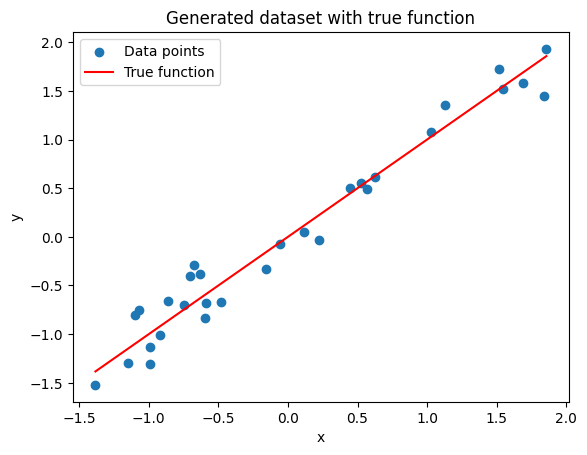
-1.4802973661668754e-17
[-0.73679458  0.60118835]

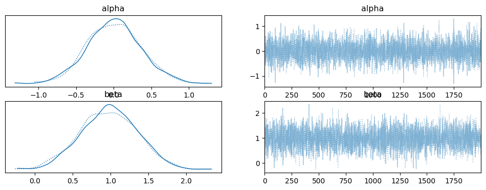
### LINEAR MODEL

with pm.Model() as model_l:
    # Priors for unknown model parameters
    alpha = pm.Normal('alpha', mu=0, sigma=10)
    beta = pm.Normal('beta', mu=0, sigma=10)

    # Linear model
    y_est = alpha + beta * x

    # Likelihood (sampling distribution) of observations
    y_obs = pm.Normal('y_obs', mu=y_est, sigma=2, observed=y)

    # Inference
    idata_l = pm.sample(2000)
    trace_l = pm.sample(return_inferencedata=False)

100.00% [3000/3000 00:02<00:00 Sampling chain 0, 0 divergences]

100.00% [3000/3000 00:02<00:00 Sampling chain 1, 0 divergences]

100.00% [2000/2000 00:02<00:00 Sampling chain 0, 0 divergences]

100.00% [2000/2000 00:01<00:00 Sampling chain 1, 0 divergences]

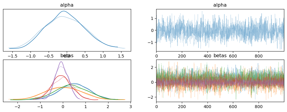
az.plot_trace(idata_l)
plt.show()

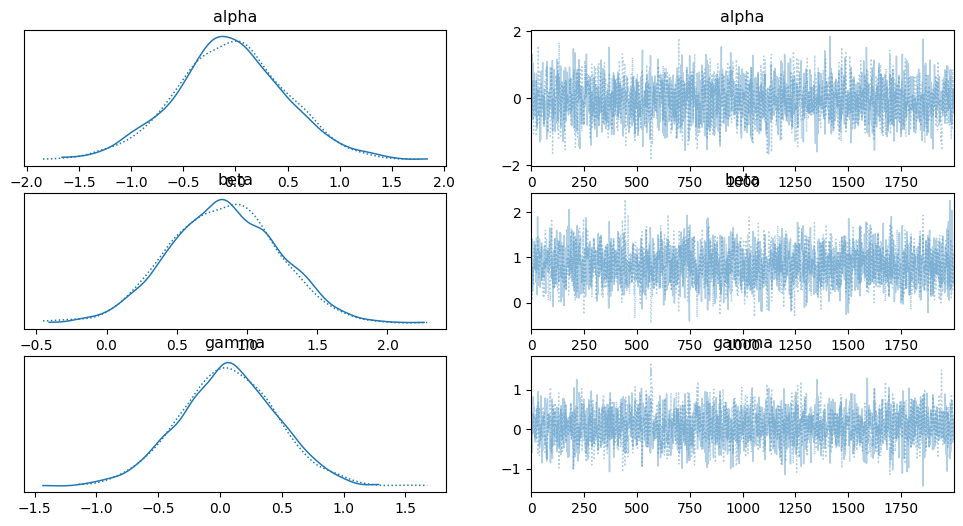
### POLYNOMIAL (ORDER 2) MODEL

with pm.Model() as model_p2:
    # Priors for unknown model parameters
    alpha = pm.Normal('alpha', mu=0, sigma=10)
    beta = pm.Normal('beta', mu=0, sigma=1)
    gamma = pm.Normal('gamma', mu=0, sigma=1)

    # Quadratic model
    y_est = alpha + beta * x + gamma * x**2

    # Likelihood (sampling distribution) of observations
    y_obs = pm.Normal('y_obs', mu=y_est, sigma=2, observed=y)

    # Inference
    idata_p2 = pm.sample(2000)

az.plot_trace(idata_p2)
#plt.show()

100.00% [3000/3000 00:03<00:00 Sampling chain 0, 0 divergences]

100.00% [3000/3000 00:04<00:00 Sampling chain 1, 0 divergences]

array([[<Axes: title={'center': 'alpha'}>,
        <Axes: title={'center': 'alpha'}>],
       [<Axes: title={'center': 'beta'}>,
        <Axes: title={'center': 'beta'}>],
       [<Axes: title={'center': 'gamma'}>,
        <Axes: title={'center': 'gamma'}>]], dtype=object)

### POLYNOMIAL (ORDER 5) MODEL

with pm.Model() as model_p5:
    # Priors for unknown model parameters
    alpha = pm.Normal('alpha', mu=0, sigma=10)
    betas = pm.Normal('betas', mu=0, sigma=1, shape = 5)

    # Quadratic model
    y_est = alpha + betas[0] * x + betas[1] * x**2 + betas[2] * x**3 + betas[3] * x**4 + betas[4] * x**5

    # Likelihood (sampling distribution) of observations
    y_obs = pm.Normal('y_obs', mu=y_est, sigma=2, observed=y)

    # Inference
    idata_p5 = pm.sample(1000)

az.plot_trace(idata_p5)
#plt.show()

100.00% [2000/2000 00:11<00:00 Sampling chain 0, 0 divergences]

100.00% [2000/2000 00:11<00:00 Sampling chain 1, 0 divergences]

array([[<Axes: title={'center': 'alpha'}>,
        <Axes: title={'center': 'alpha'}>],
       [<Axes: title={'center': 'betas'}>,
        <Axes: title={'center': 'betas'}>]], dtype=object)

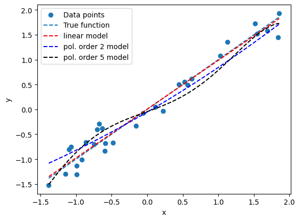
### Compare models


plt.scatter(x, y, label='Data points')
plt.plot(np.sort(x), np.sort(x), label='True function', color='C0', linestyle='--')

x_new = np.linspace(np.min(x),np.max(x),100)

#linear
alpha_l_post = idata_l.posterior['alpha'].mean(axis=0).mean(axis=0).values
beta_l_post = idata_l.posterior['beta'].mean(axis=0).mean(axis=0).values
yl_post = alpha_l_post + beta_l_post * x_new
plt.plot(x_new, yl_post, 'r', label='linear model', linestyle='--')

#pol 2
alpha_p2_post = idata_p2.posterior['alpha'].mean(axis=0).mean(axis=0).values
beta_p2_post = idata_p2.posterior['beta'].mean(axis=0).mean(axis=0).values
gamma_p2_post = idata_p2.posterior['gamma'].mean(axis=0).mean(axis=0).values
yp2_post = alpha_p2_post + beta_p2_post * x_new + gamma_p2_post * x_new**2
plt.plot(x_new, yp2_post, 'b', label='pol. order 2 model', linestyle='--')

#pol 5
alpha_p5_post = idata_p5.posterior['alpha'].mean(axis=0).mean(axis=0).values
beta1_p5_post = idata_p5.posterior['betas'].mean(axis=0)[:,0].mean(axis=0).values
beta2_p5_post = idata_p5.posterior['betas'].mean(axis=0)[:,1].mean(axis=0).values
beta3_p5_post = idata_p5.posterior['betas'].mean(axis=0)[:,2].mean(axis=0).values
beta4_p5_post = idata_p5.posterior['betas'].mean(axis=0)[:,3].mean(axis=0).values
beta5_p5_post = idata_p5.posterior['betas'].mean(axis=0)[:,4].mean(axis=0).values
yp5_post = alpha_p5_post + beta1_p5_post * x_new + beta2_p5_post * x_new**2 +  beta3_p5_post * x_new**3 \
+ beta4_p5_post * x_new**4 + beta5_p5_post * x_new**5

plt.plot(x_new, yp5_post, 'k', label='pol. order 5 model', linestyle='--')

plt.legend()
plt.xlabel('x')
plt.ylabel('y')

plt.show()

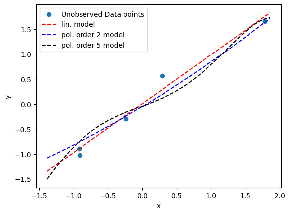
### new data points

unobserved = 5

x_unobs = np.random.uniform(-2.5, 2.5, unobserved)  # 30 random points between -5 and 5

y_unobs = x_unobs + np.random.normal(0, 0.4, unobserved)  # Adding some Gaussian noise

y_unobs =(y_unobs-np.mean(y_unobs))/np.std(y_unobs)
x_unobs =(x_unobs-np.mean(x_unobs))/np.std(x_unobs)

plt.scatter(x_unobs, y_unobs, label='Unobserved Data points')

plt.plot(x_new, yl_post, 'r', label='lin. model', linestyle='--')
plt.plot(x_new, yp2_post, 'b', label='pol. order 2 model', linestyle='--')
plt.plot(x_new, yp5_post, 'k', label='pol. order 5 model', linestyle='--')

plt.legend()
plt.xlabel('x')
plt.ylabel('y')

plt.show()

Using Posterior Predictive Checks#

y_l = pm.sample_posterior_predictive(idata_l,model=model_l)

100.00% [4000/4000 00:00<00:00]

y_p2 = pm.sample_posterior_predictive(idata_p2,model=model_p2)

100.00% [4000/4000 00:00<00:00]

y_p5 = pm.sample_posterior_predictive(idata_p5,model=model_p5)

100.00% [2000/2000 00:00<00:00]

y_l_obs = y_l.posterior_predictive['y_obs']
y_p2_obs = y_p2.posterior_predictive['y_obs']
y_p5_obs = y_p5.posterior_predictive['y_obs']

import xarray as xr
y_l_concatenated = xr.concat([y_l_obs.sel(chain=0), y_l_obs.sel(chain=1)], dim='draw')
y_p2_concatenated = xr.concat([y_p2_obs.sel(chain=0), y_p2_obs.sel(chain=1)], dim='draw')
y_p5_concatenated = xr.concat([y_p5_obs.sel(chain=0), y_p5_obs.sel(chain=1)], dim='draw')

plt.figure(figsize=(8,3))

y_o   = y
y_lo  = y_l.posterior_predictive['y_obs'].mean(axis=0).mean(axis=0).values
y_lo2 = y_l_concatenated.mean(axis=0).values #same thing as above...
y_p2o = y_p2.posterior_predictive['y_obs'].mean(axis=0).mean(axis=0).values
y_p5o = y_p5.posterior_predictive['y_obs'].mean(axis=0).mean(axis=0).values
y_p5o2 = y_p5_concatenated.mean(axis=0).values #same thing as above...


data = [y_o, y_lo, y_lo, y_p2o, y_p5o, y_p5o2]
labels = ['data', 'linear model', 'linear model conc.', 'pol. order 2', 'pol. order 5', 'pol. order 5 conc.']

for i, d in enumerate(data):
  mean = d.mean()
  err = np.percentile(d, [25,75])
  plt.errorbar(mean,-i,xerr=[[-err[0]],[err[1]]], fmt='o')
  plt.text(mean,-i+0.2, labels[i], ha='center', fontsize=14)

plt.ylim([-i-0.5,0.5])
plt.yticks([])

([], [])

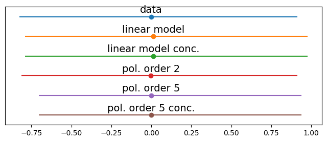
some little difference, worth exploring…

# to be completed... this code snippet can be easily extended to include other metrics, such as IQR (Q3-Q1)

fig, ax = plt.subplots(1,2,figsize=(10,3),constrained_layout=True)

labels = ['linear', 'poly2', 'poly5']

for idx, func in enumerate([np.mean]):

  T_obs = func(y)
  ax[idx].axvline(T_obs, 0, 1, color='k', ls='--')

  for label, d_sim, c in zip(labels,[y_l_concatenated.values, y_p2_concatenated.values, y_p5_concatenated.values],['C0','C1','C2']):
    T_sim = func(d_sim, 1)

    p_value = np.mean(T_sim >= T_obs)
    az.plot_kde(T_sim, plot_kwargs={'color':c}, label=f'p-value {p_value:.2f}', ax=ax[idx])

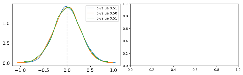
if data and simulation agree, we should expect a p-value around 0.5

Using Information Criteria#

with model_l:
    pm.compute_log_likelihood(idata_l)

100.00% [4000/4000 00:00<00:00]

with model_p2:
    pm.compute_log_likelihood(idata_p2)

100.00% [4000/4000 00:00<00:00]

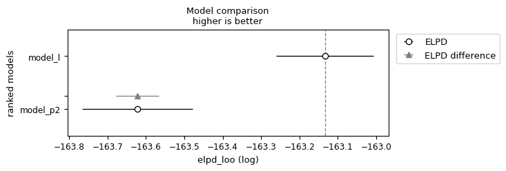
df_compare = az.compare({"model_l": idata_l, "model_p2": idata_p2}, ic='waic') #loo is recommended
df_compare

	rank	elpd_waic	p_waic	elpd_diff	weight	se	dse	warning	scale
model_l	0	-163.133370	0.061837	0.000000	1.0	0.126895	0.000000	False	log
model_p2	1	-163.621849	0.109620	0.488479	0.0	0.143890	0.055853	False	log

az.plot_compare(df_compare, insample_dev=False)

<Axes: title={'center': 'Model comparison\nhigher is better'}, xlabel='elpd_loo (log)', ylabel='ranked models'>

Bayesian Reasoning in Data Science (DATA 644)

Model Comparison

Contents

Model Comparison#

The Toy-Model#

Using Posterior Predictive Checks#

Using Information Criteria#