- bokeh
- numpy
- scipy
- matplotlib
Bayesian A/B testing
Examples of applications: Conversion Rates of Websites or Control/Treatment in Clinical Trials.
by: R. Gupta, CF (Bayesian Reasoning in Data Science, AY 2022)
Who can use this script?
Anyone running an A/B testing like website designs (conversion rates)

or similar problems like clinical trials with treatment and control groups.
App Description:
This webapp runs probabilistic programming. It utilizes PyScript, which allows to run this script directly on your browser!
It strongly relies on Lectures 1, 21 from the Bayesian Reasoning in Data Science course
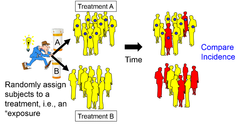
In what follows we will refer to the website design problem:
B is the standard design (or control group for a standard treatment), and A is the new design (or treatment group in a clinical trial).
alpha par (prior A)=
10
beta par (prior A)=
10
alpha par (prior B)=
10
beta par (prior B)=
10
Visitors to A (Treatment Group)=
10
Conversions from A=
5
Visitors to B (Control Group)=
10
Conversions from B=
5
from pyodide import create_proxy
@create_proxy
def on_click(evt):
pr_alphaA = Element('input_box_alphaA').element.value
if pr_alphaA == "":
pr_alphaA = 1
pr_betaA = Element('input_box_betaA').element.value
if pr_betaA == "":
pr_betaA = 1
pr_alphaB = Element('input_box_alphaB').element.value
if pr_alphaB == "":
pr_alphaB = 1
pr_betaB = Element('input_box_betaB').element.value
if pr_betaB == "":
pr_betaB = 1
vA = Element('input_box_vA').element.value
if vA == "":
vA = 127
vB = Element('input_box_vB').element.value
if vB == "":
vB = 130
cA = Element('input_box_cA').element.value
if cA == "":
cA = 22
cB = Element('input_box_cB').element.value
if cB == "":
cB = 12
run_model(pr_alphaA,pr_betaA,pr_alphaB,pr_betaB,vA,vB,cA,cB)
Made using PyScript, PyMC, Arviz, Bokeh, SciPy.
If you want to use a vague prior, leave the parameters of the Beta Distributions for the design A and B to their default values, i.e. (1,1) for both.
Otherwise, tune the parameters in such a way to represent your prior belief on designs A and B.
Sampling will take a couple of seconds.
The resulting posterior belief into what
the increase in conversion rate will be will appear below...
import warnings
warnings.filterwarnings("ignore")
import json
from js import Bokeh, JSON
from bokeh.embed import json_item
from bokeh.plotting import figure
#import arviz as az
#az.rcParams["plot.backend"] = "bokeh"
import os, sys
import numpy as np
from scipy import stats
import matplotlib.pyplot as plt
import matplotlib.tri as tri
sys.stderr = open(os.devnull, "w")
def relative_increase(a,b):
assert b!=0, "denominator is 0"
return (a-b)/b
def run_dummy(vA, vB, cA, cB):
Element("out-cA").element.innerHTML = cA
Element("out-cB").element.innerHTML = cB
Element("out-vA").element.innerHTML = vA
Element("out-vB").element.innerHTML = vB
def run_model(pr_alphaA, pr_betaA, pr_alphaB, pr_betaB, vA, vB, cA, cB):
visitors_to_A = int(vA)
visitors_to_B = int(vB)
conversions_from_A = int(cA)
conversions_from_B = int(cB)
alpha_priorA = int(pr_alphaA)
beta_priorA = int(pr_betaA)
alpha_priorB = int(pr_alphaB)
beta_priorB = int(pr_betaB)
samples = 30000
posterior_A = stats.beta(alpha_priorA+conversions_from_A,beta_priorA+visitors_to_A-conversions_from_A)
posterior_B = stats.beta(alpha_priorB+conversions_from_B,beta_priorB+visitors_to_B-conversions_from_B)
samples_posterior_A = posterior_A.rvs(samples)
samples_posterior_B = posterior_B.rvs(samples)
samples_diff = samples_posterior_A - samples_posterior_B
posterior_rel_increase = np.divide(samples_diff,samples_posterior_B)
posterior_better = samples_diff
res_10 = np.round((posterior_rel_increase>0.1).mean(),3)
res_20 = np.round((posterior_rel_increase>0.2).mean(),3)
res_50 = np.round((posterior_rel_increase>0.5).mean(),3)
A_betterthan_B = np.round((posterior_better>0.).mean(),3)
#Element("out-vA").element.innerHTML = vA
#Element("out-vB").element.innerHTML = vB
#Element("out-cA").element.innerHTML = cA
#Element("out-cB").element.innerHTML = cB
str_10 = "Probability that a relative increase is more than 10%: "+str(res_10)
str_20 = "Probability that a relative increase is more than 20%: "+str(res_20)
str_50 = "Probability that a relative increase is more than 50%: "+str(res_50)
str_better = "Probability that A is better than B: "+str(A_betterthan_B)
Element("out-res_10").element.innerHTML = str_10
Element("out-res_20").element.innerHTML = str_20
Element("out-res_50").element.innerHTML = str_50
Element("out-better").element.innerHTML = str_better
#---------------- plotting ---------------#
"""
p = figure(plot_width=400, plot_height=400)
# add a circle renderer with x and y coordinates, size, color, and alpha
p.circle([1, 2, 3, 4, 5], [6, 7, 2, 4, 5], size=15, line_color="navy", fill_color="orange", fill_alpha=0.5)
#p_json = json.dumps(json_item(p, "myplot1"))
#Bokeh.embed.embed_item(JSON.parse(p_json))
"""
#--- prior
f_pr = plt.figure()
ax = plt.subplot(121)
f_pr.set_figwidth(5)
f_pr.set_figheight(2)
x = np.linspace(0, 1, 100)
y = stats.beta(alpha_priorA, beta_priorA).pdf(x)
plt.plot(x, y,label="prior A")
#plt.xlabel('probability')
#plt.ylabel('density (prior)')
plt.legend(loc="upper right")
ax = plt.subplot(122)
f_pr.set_figwidth(5)
f_pr.set_figheight(2)
x = np.linspace(0, 1, 100)
y = stats.beta(alpha_priorB, beta_priorB).pdf(x)
plt.plot(x, y,label="prior B")
#plt.xlabel('probability')
#plt.ylabel('density (prior)')
plt.legend(loc="upper right")
pyscript.write("myplot1",f_pr)
#--- histogram of posteriors
f_post = plt.figure()
ax = plt.subplot(311)
plt.xlim(0, .5)
plt.hist(samples_posterior_A, histtype='stepfilled', bins=25, alpha=0.85,
label="posterior of $p_A$", color="#A60628", density=True)
#plt.vlines(true_p_A, 0, 80, linestyle="--", label="true $p_A$ (unknown)")
plt.legend(loc="upper right")
plt.title("Posterior distributions of $p_A$, $p_B$, and delta unknowns")
ax = plt.subplot(312)
plt.xlim(0, .5)
plt.hist(samples_posterior_B, histtype='stepfilled', bins=25, alpha=0.85,
label="posterior of $p_B$", color="#467821", density=True)
#plt.vlines(true_p_B, 0, 80, linestyle="--", label="true $p_B$ (unknown)")
plt.legend(loc="upper right")
ax = plt.subplot(313)
plt.hist(samples_diff, histtype='stepfilled', bins=30, alpha=0.85,
label="posterior of delta", color="#7A68A6", density=True)
#plt.vlines(true_p_A - true_p_B, 0, 60, linestyle="--",
# label="true delta (unknown)")
plt.vlines(0, 0, 60, color="black", alpha=0.2)
plt.legend(loc="upper right")
pyscript.write("myplot2",f_post)
pr_alphaA = Element('input_box_alphaA').element.value
pr_betaA = Element('input_box_betaA').element.value
vA = Element('input_box_vA').element.value
vB = Element('input_box_vB').element.value
cA = Element('input_box_cA').element.value
cB = Element('input_box_cB').element.value