Bayes Factors

Based on https://www.pymc.io/projects/examples/en/latest/diagnostics_and_criticism/Bayes_factor.html

%pip install pymc pytensor

Requirement already satisfied: pymc in /usr/local/lib/python3.10/dist-packages (5.10.4)
Requirement already satisfied: pytensor in /usr/local/lib/python3.10/dist-packages (2.18.6)
Requirement already satisfied: arviz>=0.13.0 in /usr/local/lib/python3.10/dist-packages (from pymc) (0.15.1)
Requirement already satisfied: cachetools>=4.2.1 in /usr/local/lib/python3.10/dist-packages (from pymc) (5.3.3)
Requirement already satisfied: cloudpickle in /usr/local/lib/python3.10/dist-packages (from pymc) (2.2.1)
Requirement already satisfied: fastprogress>=0.2.0 in /usr/local/lib/python3.10/dist-packages (from pymc) (1.0.3)
Requirement already satisfied: numpy>=1.15.0 in /usr/local/lib/python3.10/dist-packages (from pymc) (1.25.2)
Requirement already satisfied: pandas>=0.24.0 in /usr/local/lib/python3.10/dist-packages (from pymc) (1.5.3)
Requirement already satisfied: scipy>=1.4.1 in /usr/local/lib/python3.10/dist-packages (from pymc) (1.11.4)
Requirement already satisfied: typing-extensions>=3.7.4 in /usr/local/lib/python3.10/dist-packages (from pymc) (4.10.0)
Requirement already satisfied: setuptools>=48.0.0 in /usr/local/lib/python3.10/dist-packages (from pytensor) (67.7.2)
Requirement already satisfied: filelock in /usr/local/lib/python3.10/dist-packages (from pytensor) (3.13.1)
Requirement already satisfied: etuples in /usr/local/lib/python3.10/dist-packages (from pytensor) (0.3.9)
Requirement already satisfied: logical-unification in /usr/local/lib/python3.10/dist-packages (from pytensor) (0.4.6)
Requirement already satisfied: miniKanren in /usr/local/lib/python3.10/dist-packages (from pytensor) (1.0.3)
Requirement already satisfied: cons in /usr/local/lib/python3.10/dist-packages (from pytensor) (0.4.6)
Requirement already satisfied: matplotlib>=3.2 in /usr/local/lib/python3.10/dist-packages (from arviz>=0.13.0->pymc) (3.7.1)
Requirement already satisfied: packaging in /usr/local/lib/python3.10/dist-packages (from arviz>=0.13.0->pymc) (23.2)
Requirement already satisfied: xarray>=0.21.0 in /usr/local/lib/python3.10/dist-packages (from arviz>=0.13.0->pymc) (2023.7.0)
Requirement already satisfied: h5netcdf>=1.0.2 in /usr/local/lib/python3.10/dist-packages (from arviz>=0.13.0->pymc) (1.3.0)
Requirement already satisfied: xarray-einstats>=0.3 in /usr/local/lib/python3.10/dist-packages (from arviz>=0.13.0->pymc) (0.7.0)
Requirement already satisfied: python-dateutil>=2.8.1 in /usr/local/lib/python3.10/dist-packages (from pandas>=0.24.0->pymc) (2.8.2)
Requirement already satisfied: pytz>=2020.1 in /usr/local/lib/python3.10/dist-packages (from pandas>=0.24.0->pymc) (2023.4)
Requirement already satisfied: toolz in /usr/local/lib/python3.10/dist-packages (from logical-unification->pytensor) (0.12.1)
Requirement already satisfied: multipledispatch in /usr/local/lib/python3.10/dist-packages (from logical-unification->pytensor) (1.0.0)
Requirement already satisfied: h5py in /usr/local/lib/python3.10/dist-packages (from h5netcdf>=1.0.2->arviz>=0.13.0->pymc) (3.9.0)
Requirement already satisfied: contourpy>=1.0.1 in /usr/local/lib/python3.10/dist-packages (from matplotlib>=3.2->arviz>=0.13.0->pymc) (1.2.0)
Requirement already satisfied: cycler>=0.10 in /usr/local/lib/python3.10/dist-packages (from matplotlib>=3.2->arviz>=0.13.0->pymc) (0.12.1)
Requirement already satisfied: fonttools>=4.22.0 in /usr/local/lib/python3.10/dist-packages (from matplotlib>=3.2->arviz>=0.13.0->pymc) (4.49.0)
Requirement already satisfied: kiwisolver>=1.0.1 in /usr/local/lib/python3.10/dist-packages (from matplotlib>=3.2->arviz>=0.13.0->pymc) (1.4.5)
Requirement already satisfied: pillow>=6.2.0 in /usr/local/lib/python3.10/dist-packages (from matplotlib>=3.2->arviz>=0.13.0->pymc) (9.4.0)
Requirement already satisfied: pyparsing>=2.3.1 in /usr/local/lib/python3.10/dist-packages (from matplotlib>=3.2->arviz>=0.13.0->pymc) (3.1.1)
Requirement already satisfied: six>=1.5 in /usr/local/lib/python3.10/dist-packages (from python-dateutil>=2.8.1->pandas>=0.24.0->pymc) (1.16.0)

import arviz as az
import numpy as np
import pymc as pm

from matplotlib import pyplot as plt
from matplotlib.ticker import FormatStrFormatter
from scipy.special import betaln
from scipy.stats import beta

print(f"Running on PyMC v{pm.__version__}")

Running on PyMC v5.10.4

Let’s consider the coin flipping problem, and let’s use the Binomial/Beta model.

Let’s consider two priors, with parameters (1,1) and (30,30) for α and β

y = np.repeat([1, 0], [50, 50])  # 50 "heads" and 50 "tails" # NOTICE THIS MEANS WE HAVE A FAIR COIN!
priors = ((1, 1), (30, 30)) # What model is going to be best?

models = []
idatas = []
for alpha, beta in priors:
    with pm.Model() as model:
        a = pm.Beta("a", alpha, beta)
        yl = pm.Bernoulli("yl", a, observed=y)
        idata = pm.sample_smc(random_seed=42)
        models.append(model)
        idatas.append(idata)

100.00% [200/200 00:00<? Chain: 2/2 Stage: 2 Beta: 1.000]

100.00% [200/200 00:00<? Chain: 2/2 Stage: 0 Beta: 1.000]

/usr/local/lib/python3.10/dist-packages/arviz/data/base.py:221: UserWarning: More chains (2) than draws (1). Passed array should have shape (chains, draws, *shape)
  warnings.warn(

Let’s calculate the Bayes factors

BF_smc = np.exp(
    idatas[1].sample_stats["log_marginal_likelihood"].mean()
    - idatas[0].sample_stats["log_marginal_likelihood"].mean()
)
np.round(BF_smc).item()

5.0

We see that the model with the more concentrated prior beta(30,30) has \(\sim\)5 times more support than the model with the more extended prior beta(1,1).

Besides the exact numerical value this should not be surprising since the prior for the most favoured model is concentrated around \(\theta=\)0.5 and the data has equal number of head and tails, consistent with a value of \(\theta\) around 0.5.

Bayes Factor and Inference

So far we have used Bayes factors to judge which model seems to be better at explaining the data, and we get that one of the models is \(\approx\) 5 times better than the other.

But what about the posterior we get from these models? How different they are?

az.summary(idatas[0], var_names="a", kind="stats").round(2)

	mean	sd	hdi_3%	hdi_97%
a	0.5	0.05	0.41	0.59

az.summary(idatas[1], var_names="a", kind="stats").round(2)

	mean	sd	hdi_3%	hdi_97%
a	0.5	0.04	0.42	0.57

We may argue that the results are pretty similar, we have the same mean value for \(\theta\), and a slightly wider posterior for model_0, as expected since this model has a wider prior. We can also check the posterior predictive distribution to see how similar they are.

ppc_0 = pm.sample_posterior_predictive(idatas[0], model=models[0]).posterior_predictive
ppc_1 = pm.sample_posterior_predictive(idatas[1], model=models[1]).posterior_predictive

100.00% [4000/4000 00:01<00:00]

100.00% [4000/4000 00:02<00:00]

ppc_0

<xarray.Dataset>
Dimensions:   (chain: 2, draw: 2000, yl_dim_2: 100)
Coordinates:
  * chain     (chain) int64 0 1
  * draw      (draw) int64 0 1 2 3 4 5 6 ... 1993 1994 1995 1996 1997 1998 1999
  * yl_dim_2  (yl_dim_2) int64 0 1 2 3 4 5 6 7 8 ... 91 92 93 94 95 96 97 98 99
Data variables:
    yl        (chain, draw, yl_dim_2) int64 1 1 0 1 0 1 0 1 ... 0 0 0 1 0 0 1 1
Attributes:
    created_at:                 2024-03-07T18:21:05.727051
    arviz_version:              0.15.1
    inference_library:          pymc
    inference_library_version:  5.10.4

xarray.Dataset

• Dimensions:
  • chain: 2
  • draw: 2000
  • yl_dim_2: 100
• Coordinates: (3)
  • chain
    (chain)
    int64
    0 1

    array([0, 1])

  • draw
    (draw)
    int64
    0 1 2 3 4 ... 1996 1997 1998 1999

    array([   0,    1,    2, ..., 1997, 1998, 1999])

  • yl_dim_2
    (yl_dim_2)
    int64
    0 1 2 3 4 5 6 ... 94 95 96 97 98 99

    array([ 0,  1,  2,  3,  4,  5,  6,  7,  8,  9, 10, 11, 12, 13, 14, 15, 16, 17,
           18, 19, 20, 21, 22, 23, 24, 25, 26, 27, 28, 29, 30, 31, 32, 33, 34, 35,
           36, 37, 38, 39, 40, 41, 42, 43, 44, 45, 46, 47, 48, 49, 50, 51, 52, 53,
           54, 55, 56, 57, 58, 59, 60, 61, 62, 63, 64, 65, 66, 67, 68, 69, 70, 71,
           72, 73, 74, 75, 76, 77, 78, 79, 80, 81, 82, 83, 84, 85, 86, 87, 88, 89,
           90, 91, 92, 93, 94, 95, 96, 97, 98, 99])

• Data variables: (1)
  • yl
    (chain, draw, yl_dim_2)
    int64
    1 1 0 1 0 1 0 1 ... 0 0 0 1 0 0 1 1

    array([[[1, 1, 0, ..., 0, 1, 1],
            [0, 1, 1, ..., 0, 0, 1],
            [0, 1, 1, ..., 1, 1, 1],
            ...,
            [0, 1, 0, ..., 0, 0, 0],
            [1, 0, 0, ..., 0, 1, 0],
            [1, 0, 0, ..., 0, 1, 1]],
    
           [[1, 0, 0, ..., 0, 1, 1],
            [1, 1, 0, ..., 0, 0, 1],
            [0, 1, 0, ..., 0, 0, 1],
            ...,
            [1, 1, 0, ..., 0, 1, 0],
            [0, 1, 0, ..., 0, 0, 1],
            [0, 0, 1, ..., 0, 1, 1]]])

• Indexes: (3)
  • chain
    PandasIndex

    PandasIndex(Int64Index([0, 1], dtype='int64', name='chain'))

  • draw
    PandasIndex

    PandasIndex(Int64Index([   0,    1,    2,    3,    4,    5,    6,    7,    8,    9,
                ...
                1990, 1991, 1992, 1993, 1994, 1995, 1996, 1997, 1998, 1999],
               dtype='int64', name='draw', length=2000))

  • yl_dim_2
    PandasIndex

    PandasIndex(Int64Index([ 0,  1,  2,  3,  4,  5,  6,  7,  8,  9, 10, 11, 12, 13, 14, 15, 16,
                17, 18, 19, 20, 21, 22, 23, 24, 25, 26, 27, 28, 29, 30, 31, 32, 33,
                34, 35, 36, 37, 38, 39, 40, 41, 42, 43, 44, 45, 46, 47, 48, 49, 50,
                51, 52, 53, 54, 55, 56, 57, 58, 59, 60, 61, 62, 63, 64, 65, 66, 67,
                68, 69, 70, 71, 72, 73, 74, 75, 76, 77, 78, 79, 80, 81, 82, 83, 84,
                85, 86, 87, 88, 89, 90, 91, 92, 93, 94, 95, 96, 97, 98, 99],
               dtype='int64', name='yl_dim_2'))

• Attributes: (4)

  created_at :

  2024-03-07T18:21:05.727051

  arviz_version :

  0.15.1

  inference_library :

  pymc

  inference_library_version :

  5.10.4

_, ax = plt.subplots(figsize=(9, 6))

bins = np.linspace(0.2, 0.8, 8)

# Computes the mean of the "yl" variable across a specific dimension, "yl_dim_2"
ax = az.plot_dist(
    ppc_0["yl"].mean("yl_dim_2"),
    label="model_0",
    kind="hist",
    hist_kwargs={"alpha": 0.5, "bins": bins},
)


ax = az.plot_dist(
    ppc_1["yl"].mean("yl_dim_2"),
    label="model_1",
    color="C1",
    kind="hist",
    hist_kwargs={"alpha": 0.5, "bins": bins},
    ax=ax,
)
ax.legend()
ax.set_xlabel("$\\theta$")
ax.xaxis.set_major_formatter(FormatStrFormatter("%0.1f"))
ax.set_yticks([]);

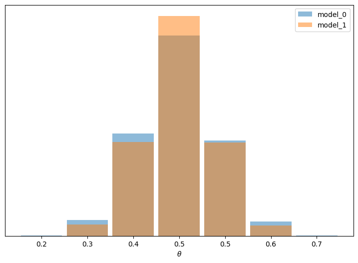
In this example the observed data is more consistent with model_1 (because the prior is concentrated around the correct value of \(\theta\) ) than model_0 (which assigns equal probability to every possible value of \(\theta\)), and this difference is captured by the Bayes factor.

We could say Bayes factors are measuring which model, as a whole, is better, including details of the prior that may be irrelevant for parameter inference. In fact in this example we can also see that it is possible to have two different models, with different Bayes factors, but nevertheless get very similar predictions.

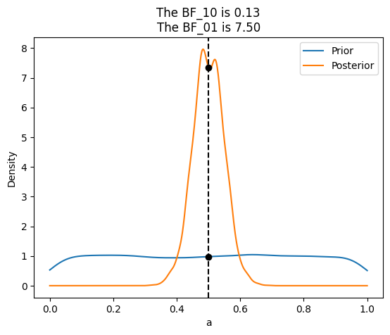
Savage-Dickey Density Ratio

For the previous examples we have compared two beta-binomial models, but sometimes what we want to do is to compare a null hypothesis H_0 (or null model) against an alternative one H_1. For example, to answer the question is this coin biased?, we could compare the value \(\theta=\)0.5 (representing no bias) against the result from a model were we let \(\theta\) to vary. For this kind of comparison the null-model is nested within the alternative, meaning the null is a particular value of the model we are building. In those cases computing the Bayes Factor is very easy and it does not require any special method, because the math works out conveniently so we just need to compare the prior and posterior evaluated at the null-value (for example \(\theta=0.5\)), under the alternative model. We can see that is true from the following expression:

\(BF_{01} = \frac{P(y|H_{0})}{P(y|H_{1})}=\frac{P(\theta=\theta_{0}|y,H_{1})}{P(\theta=\theta_{0}|H_{1})}\)

where \(\theta_{0}=\)0.5 in our exercise.

with pm.Model() as model_uni:
    a = pm.Beta("a", 1, 1)
    yl = pm.Bernoulli("yl", a, observed=y)
    idata_uni = pm.sample(2000, random_seed=42)
    idata_uni.extend(pm.sample_prior_predictive(8000))

100.00% [3000/3000 00:04<00:00 Sampling chain 0, 0 divergences]

100.00% [3000/3000 00:05<00:00 Sampling chain 1, 0 divergences]

az.plot_bf(idata_uni, var_name="a", ref_val=0.5)

({'BF10': array([0.13329301]), 'BF01': array([7.50226909])},
 <Axes: title={'center': 'The BF_10 is 0.13\nThe BF_01 is 7.50'}, xlabel='a', ylabel='Density'>)

with pm.Model() as model_conc:
    a = pm.Beta("a", 30, 30)
    yl = pm.Bernoulli("yl", a, observed=y)
    idata_conc = pm.sample(2000, random_seed=42)
    idata_conc.extend(pm.sample_prior_predictive(8000))

100.00% [3000/3000 00:02<00:00 Sampling chain 0, 0 divergences]

100.00% [3000/3000 00:02<00:00 Sampling chain 1, 0 divergences]

az.plot_bf(idata_conc, var_name="a", ref_val=0.5);

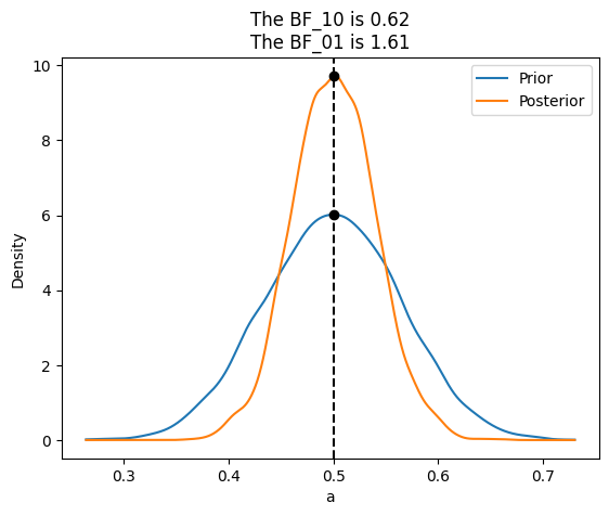
If instead our model would be a beta-binomial with prior beta(30, 30), the BF_01 would be lower (anecdotal on the Jeffreys’ scale). This is because under this model the value of \(\theta=\)0.5 is much more likely a priori than for a uniform prior, and hence the posterior and prior will me much more similar. Namely there is not too much surprise about seeing the posterior concentrated around 0.5 after collecting data.

Note:

• idata_conc.extend(pm.sample_prior_predictive(8000)) — T*his command performs prior predictive sampling by drawing 8000 samples from the prior distribution of the model (i.e., sampling from the model without considering any observed data). This helps in understanding the implications of the priors before observing any data. *

• The .extend() method is called on the idata_conc object, which originally contained the posterior samples. By using this method, the prior predictive samples are added to the idata_conc object, effectively combining both posterior and prior predictive samples in one container. This can be useful for comprehensive model diagnostics, allowing one to compare predictions made purely from priors with those adjusted by the data.

idata_conc

arviz.InferenceData

• posterior

  <xarray.Dataset>
  Dimensions:  (chain: 2, draw: 2000)
  Coordinates:
    * chain    (chain) int64 0 1
    * draw     (draw) int64 0 1 2 3 4 5 6 7 ... 1993 1994 1995 1996 1997 1998 1999
  Data variables:
      a        (chain, draw) float64 0.5302 0.5308 0.5308 ... 0.5508 0.5382 0.5382
  Attributes:
      created_at:                 2024-03-07T18:35:13.998346
      arviz_version:              0.15.1
      inference_library:          pymc
      inference_library_version:  5.10.4
      sampling_time:              4.5322511196136475
      tuning_steps:               1000

  xarray.Dataset

  • Dimensions:
    • chain: 2
    • draw: 2000
  • Coordinates: (2)
    • chain
      (chain)
      int64
      0 1

      array([0, 1])

    • draw
      (draw)
      int64
      0 1 2 3 4 ... 1996 1997 1998 1999

      array([   0,    1,    2, ..., 1997, 1998, 1999])

  • Data variables: (1)
    • a
      (chain, draw)
      float64
      0.5302 0.5308 ... 0.5382 0.5382

      array([[0.53017054, 0.5308187 , 0.5308187 , ..., 0.46887635, 0.46887635,
              0.54472053],
             [0.56926711, 0.56926711, 0.52816491, ..., 0.55077776, 0.53817355,
              0.53817355]])

  • Indexes: (2)
    • chain
      PandasIndex

      PandasIndex(Int64Index([0, 1], dtype='int64', name='chain'))

    • draw
      PandasIndex

      PandasIndex(Int64Index([   0,    1,    2,    3,    4,    5,    6,    7,    8,    9,
                  ...
                  1990, 1991, 1992, 1993, 1994, 1995, 1996, 1997, 1998, 1999],
                 dtype='int64', name='draw', length=2000))

  • Attributes: (6)

    created_at :

    2024-03-07T18:35:13.998346

    arviz_version :

    0.15.1

    inference_library :

    pymc

    inference_library_version :

    5.10.4

    sampling_time :

    4.5322511196136475

    tuning_steps :

    1000

  
  
• sample_stats

  <xarray.Dataset>
  Dimensions:                (chain: 2, draw: 2000)
  Coordinates:
    * chain                  (chain) int64 0 1
    * draw                   (draw) int64 0 1 2 3 4 5 ... 1995 1996 1997 1998 1999
  Data variables: (12/17)
      perf_counter_diff      (chain, draw) float64 0.0004967 ... 0.0002471
      energy_error           (chain, draw) float64 0.08762 0.005578 ... 0.0
      step_size_bar          (chain, draw) float64 1.273 1.273 ... 1.414 1.414
      diverging              (chain, draw) bool False False False ... False False
      step_size              (chain, draw) float64 1.16 1.16 1.16 ... 1.393 1.393
      max_energy_error       (chain, draw) float64 0.08762 0.005578 ... 3.263
      ...                     ...
      n_steps                (chain, draw) float64 3.0 1.0 1.0 3.0 ... 1.0 1.0 1.0
      energy                 (chain, draw) float64 69.21 69.32 ... 69.77 72.84
      reached_max_treedepth  (chain, draw) bool False False False ... False False
      smallest_eigval        (chain, draw) float64 nan nan nan nan ... nan nan nan
      process_time_diff      (chain, draw) float64 0.0004974 ... 0.000247
      acceptance_rate        (chain, draw) float64 0.9539 0.9944 ... 1.0 0.03826
  Attributes:
      created_at:                 2024-03-07T18:35:14.014844
      arviz_version:              0.15.1
      inference_library:          pymc
      inference_library_version:  5.10.4
      sampling_time:              4.5322511196136475
      tuning_steps:               1000

  xarray.Dataset

  • Dimensions:
    • chain: 2
    • draw: 2000
  • Coordinates: (2)
    • chain
      (chain)
      int64
      0 1

      array([0, 1])

    • draw
      (draw)
      int64
      0 1 2 3 4 ... 1996 1997 1998 1999

      array([   0,    1,    2, ..., 1997, 1998, 1999])

  • Data variables: (17)
    • perf_counter_diff
      (chain, draw)
      float64
      0.0004967 0.0002335 ... 0.0002471

      array([[0.00049675, 0.00023347, 0.00033676, ..., 0.00088093, 0.00043729,
              0.00092193],
             [0.00090108, 0.00045495, 0.00043695, ..., 0.0002293 , 0.0002283 ,
              0.00024713]])

    • energy_error
      (chain, draw)
      float64
      0.08762 0.005578 ... -0.1853 0.0

      array([[ 0.08761647,  0.00557756,  0.        , ...,  0.11880747,
               0.        ,  0.14899019],
             [ 0.38762129,  0.        , -0.66306018, ...,  0.4205178 ,
              -0.18525839,  0.        ]])

    • step_size_bar
      (chain, draw)
      float64
      1.273 1.273 1.273 ... 1.414 1.414

      array([[1.27252138, 1.27252138, 1.27252138, ..., 1.27252138, 1.27252138,
              1.27252138],
             [1.41415854, 1.41415854, 1.41415854, ..., 1.41415854, 1.41415854,
              1.41415854]])

    • diverging
      (chain, draw)
      bool
      False False False ... False False

      array([[False, False, False, ..., False, False, False],
             [False, False, False, ..., False, False, False]])

    • step_size
      (chain, draw)
      float64
      1.16 1.16 1.16 ... 1.393 1.393

      array([[1.16039802, 1.16039802, 1.16039802, ..., 1.16039802, 1.16039802,
              1.16039802],
             [1.39293512, 1.39293512, 1.39293512, ..., 1.39293512, 1.39293512,
              1.39293512]])

    • max_energy_error
      (chain, draw)
      float64
      0.08762 0.005578 ... -0.1853 3.263

      array([[ 0.08761647,  0.00557756,  2.1299498 , ...,  0.71756504,
               0.92784039,  0.30757756],
             [ 0.46252791,  0.97493698, -0.66306018, ...,  0.4205178 ,
              -0.18525839,  3.2633462 ]])

    • largest_eigval
      (chain, draw)
      float64
      nan nan nan nan ... nan nan nan nan

      array([[nan, nan, nan, ..., nan, nan, nan],
             [nan, nan, nan, ..., nan, nan, nan]])

    • perf_counter_start
      (chain, draw)
      float64
      2.455e+03 2.455e+03 ... 2.459e+03

      array([[2455.18705132, 2455.18763807, 2455.1879684 , ..., 2456.70207632,
              2456.70314498, 2456.70373323],
             [2457.74375345, 2457.74481203, 2457.7454125 , ..., 2459.01615432,
              2459.01646392, 2459.01678554]])

    • index_in_trajectory
      (chain, draw)
      int64
      -1 1 0 -1 1 -2 ... 1 1 -2 -1 -1 0

      array([[-1,  1,  0, ...,  2,  0,  2],
             [ 1,  0,  1, ..., -1, -1,  0]])

    • tree_depth
      (chain, draw)
      int64
      2 1 1 2 2 2 2 1 ... 1 1 1 1 2 1 1 1

      array([[2, 1, 1, ..., 2, 1, 2],
             [2, 1, 1, ..., 1, 1, 1]])

    • lp
      (chain, draw)
      float64
      -69.18 -69.19 ... -69.35 -69.35

      array([[-69.17561325, -69.18831022, -69.18831022, ..., -69.19437808,
              -69.19437808, -69.52634775],
             [-70.43406058, -70.43406058, -69.13804538, ..., -69.71316401,
              -69.35147271, -69.35147271]])

    • n_steps
      (chain, draw)
      float64
      3.0 1.0 1.0 3.0 ... 3.0 1.0 1.0 1.0

      array([[3., 1., 1., ..., 3., 1., 3.],
             [3., 1., 1., ..., 1., 1., 1.]])

    • energy
      (chain, draw)
      float64
      69.21 69.32 72.02 ... 69.77 72.84

      array([[69.20828138, 69.31598216, 72.01860404, ..., 70.05592408,
              70.46988223, 69.99311233],
             [70.84494806, 72.19857254, 69.91045724, ..., 69.72249351,
              69.77242927, 72.83742211]])

    • reached_max_treedepth
      (chain, draw)
      bool
      False False False ... False False

      array([[False, False, False, ..., False, False, False],
             [False, False, False, ..., False, False, False]])

    • smallest_eigval
      (chain, draw)
      float64
      nan nan nan nan ... nan nan nan nan

      array([[nan, nan, nan, ..., nan, nan, nan],
             [nan, nan, nan, ..., nan, nan, nan]])

    • process_time_diff
      (chain, draw)
      float64
      0.0004974 0.0002336 ... 0.000247

      array([[0.00049743, 0.0002336 , 0.00033716, ..., 0.00088144, 0.00043764,
              0.00092221],
             [0.0009012 , 0.00045514, 0.00043743, ..., 0.00022944, 0.00022838,
              0.00024696]])

    • acceptance_rate
      (chain, draw)
      float64
      0.9539 0.9944 ... 1.0 0.03826

      array([[0.95394689, 0.99443797, 0.11884326, ..., 0.64499674, 0.39540671,
              0.81772211],
             [0.75183542, 0.37721612, 1.        , ..., 0.65670669, 1.        ,
              0.03826016]])

  • Indexes: (2)
    • chain
      PandasIndex

      PandasIndex(Int64Index([0, 1], dtype='int64', name='chain'))

    • draw
      PandasIndex

      PandasIndex(Int64Index([   0,    1,    2,    3,    4,    5,    6,    7,    8,    9,
                  ...
                  1990, 1991, 1992, 1993, 1994, 1995, 1996, 1997, 1998, 1999],
                 dtype='int64', name='draw', length=2000))

  • Attributes: (6)

    created_at :

    2024-03-07T18:35:14.014844

    arviz_version :

    0.15.1

    inference_library :

    pymc

    inference_library_version :

    5.10.4

    sampling_time :

    4.5322511196136475

    tuning_steps :

    1000

  
  
• prior

  <xarray.Dataset>
  Dimensions:  (chain: 1, draw: 8000)
  Coordinates:
    * chain    (chain) int64 0
    * draw     (draw) int64 0 1 2 3 4 5 6 7 ... 7993 7994 7995 7996 7997 7998 7999
  Data variables:
      a        (chain, draw) float64 0.5261 0.5322 0.4858 ... 0.527 0.5547 0.5833
  Attributes:
      created_at:                 2024-03-07T18:35:14.975611
      arviz_version:              0.15.1
      inference_library:          pymc
      inference_library_version:  5.10.4

  xarray.Dataset

  • Dimensions:
    • chain: 1
    • draw: 8000
  • Coordinates: (2)
    • chain
      (chain)
      int64
      0

      array([0])

    • draw
      (draw)
      int64
      0 1 2 3 4 ... 7996 7997 7998 7999

      array([   0,    1,    2, ..., 7997, 7998, 7999])

  • Data variables: (1)
    • a
      (chain, draw)
      float64
      0.5261 0.5322 ... 0.5547 0.5833

      array([[0.52608126, 0.53220475, 0.48580258, ..., 0.5270228 , 0.55467752,
              0.58332758]])

  • Indexes: (2)
    • chain
      PandasIndex

      PandasIndex(Int64Index([0], dtype='int64', name='chain'))

    • draw
      PandasIndex

      PandasIndex(Int64Index([   0,    1,    2,    3,    4,    5,    6,    7,    8,    9,
                  ...
                  7990, 7991, 7992, 7993, 7994, 7995, 7996, 7997, 7998, 7999],
                 dtype='int64', name='draw', length=8000))

  • Attributes: (4)

    created_at :

    2024-03-07T18:35:14.975611

    arviz_version :

    0.15.1

    inference_library :

    pymc

    inference_library_version :

    5.10.4

  
  
• prior_predictive

  <xarray.Dataset>
  Dimensions:   (chain: 1, draw: 8000, yl_dim_0: 100)
  Coordinates:
    * chain     (chain) int64 0
    * draw      (draw) int64 0 1 2 3 4 5 6 ... 7993 7994 7995 7996 7997 7998 7999
    * yl_dim_0  (yl_dim_0) int64 0 1 2 3 4 5 6 7 8 ... 91 92 93 94 95 96 97 98 99
  Data variables:
      yl        (chain, draw, yl_dim_0) int64 1 1 1 1 0 0 1 0 ... 1 1 1 1 0 1 1 0
  Attributes:
      created_at:                 2024-03-07T18:35:14.976794
      arviz_version:              0.15.1
      inference_library:          pymc
      inference_library_version:  5.10.4

  xarray.Dataset

  • Dimensions:
    • chain: 1
    • draw: 8000
    • yl_dim_0: 100
  • Coordinates: (3)
    • chain
      (chain)
      int64
      0

      array([0])

    • draw
      (draw)
      int64
      0 1 2 3 4 ... 7996 7997 7998 7999

      array([   0,    1,    2, ..., 7997, 7998, 7999])

    • yl_dim_0
      (yl_dim_0)
      int64
      0 1 2 3 4 5 6 ... 94 95 96 97 98 99

      array([ 0,  1,  2,  3,  4,  5,  6,  7,  8,  9, 10, 11, 12, 13, 14, 15, 16, 17,
             18, 19, 20, 21, 22, 23, 24, 25, 26, 27, 28, 29, 30, 31, 32, 33, 34, 35,
             36, 37, 38, 39, 40, 41, 42, 43, 44, 45, 46, 47, 48, 49, 50, 51, 52, 53,
             54, 55, 56, 57, 58, 59, 60, 61, 62, 63, 64, 65, 66, 67, 68, 69, 70, 71,
             72, 73, 74, 75, 76, 77, 78, 79, 80, 81, 82, 83, 84, 85, 86, 87, 88, 89,
             90, 91, 92, 93, 94, 95, 96, 97, 98, 99])

  • Data variables: (1)
    • yl
      (chain, draw, yl_dim_0)
      int64
      1 1 1 1 0 0 1 0 ... 1 1 1 1 0 1 1 0

      array([[[1, 1, 1, ..., 1, 1, 1],
              [0, 1, 1, ..., 1, 1, 1],
              [0, 0, 1, ..., 1, 0, 1],
              ...,
              [0, 0, 0, ..., 1, 0, 0],
              [0, 1, 0, ..., 1, 0, 1],
              [0, 0, 0, ..., 1, 1, 0]]])

  • Indexes: (3)
    • chain
      PandasIndex

      PandasIndex(Int64Index([0], dtype='int64', name='chain'))

    • draw
      PandasIndex

      PandasIndex(Int64Index([   0,    1,    2,    3,    4,    5,    6,    7,    8,    9,
                  ...
                  7990, 7991, 7992, 7993, 7994, 7995, 7996, 7997, 7998, 7999],
                 dtype='int64', name='draw', length=8000))

    • yl_dim_0
      PandasIndex

      PandasIndex(Int64Index([ 0,  1,  2,  3,  4,  5,  6,  7,  8,  9, 10, 11, 12, 13, 14, 15, 16,
                  17, 18, 19, 20, 21, 22, 23, 24, 25, 26, 27, 28, 29, 30, 31, 32, 33,
                  34, 35, 36, 37, 38, 39, 40, 41, 42, 43, 44, 45, 46, 47, 48, 49, 50,
                  51, 52, 53, 54, 55, 56, 57, 58, 59, 60, 61, 62, 63, 64, 65, 66, 67,
                  68, 69, 70, 71, 72, 73, 74, 75, 76, 77, 78, 79, 80, 81, 82, 83, 84,
                  85, 86, 87, 88, 89, 90, 91, 92, 93, 94, 95, 96, 97, 98, 99],
                 dtype='int64', name='yl_dim_0'))

  • Attributes: (4)

    created_at :

    2024-03-07T18:35:14.976794

    arviz_version :

    0.15.1

    inference_library :

    pymc

    inference_library_version :

    5.10.4

  
  
• observed_data

  <xarray.Dataset>
  Dimensions:   (yl_dim_0: 100)
  Coordinates:
    * yl_dim_0  (yl_dim_0) int64 0 1 2 3 4 5 6 7 8 ... 91 92 93 94 95 96 97 98 99
  Data variables:
      yl        (yl_dim_0) int64 1 1 1 1 1 1 1 1 1 1 1 1 ... 0 0 0 0 0 0 0 0 0 0 0
  Attributes:
      created_at:                 2024-03-07T18:35:14.021622
      arviz_version:              0.15.1
      inference_library:          pymc
      inference_library_version:  5.10.4

  xarray.Dataset

  • Dimensions:
    • yl_dim_0: 100
  • Coordinates: (1)
    • yl_dim_0
      (yl_dim_0)
      int64
      0 1 2 3 4 5 6 ... 94 95 96 97 98 99

      array([ 0,  1,  2,  3,  4,  5,  6,  7,  8,  9, 10, 11, 12, 13, 14, 15, 16, 17,
             18, 19, 20, 21, 22, 23, 24, 25, 26, 27, 28, 29, 30, 31, 32, 33, 34, 35,
             36, 37, 38, 39, 40, 41, 42, 43, 44, 45, 46, 47, 48, 49, 50, 51, 52, 53,
             54, 55, 56, 57, 58, 59, 60, 61, 62, 63, 64, 65, 66, 67, 68, 69, 70, 71,
             72, 73, 74, 75, 76, 77, 78, 79, 80, 81, 82, 83, 84, 85, 86, 87, 88, 89,
             90, 91, 92, 93, 94, 95, 96, 97, 98, 99])

  • Data variables: (1)
    • yl
      (yl_dim_0)
      int64
      1 1 1 1 1 1 1 1 ... 0 0 0 0 0 0 0 0

      array([1, 1, 1, 1, 1, 1, 1, 1, 1, 1, 1, 1, 1, 1, 1, 1, 1, 1, 1, 1, 1, 1,
             1, 1, 1, 1, 1, 1, 1, 1, 1, 1, 1, 1, 1, 1, 1, 1, 1, 1, 1, 1, 1, 1,
             1, 1, 1, 1, 1, 1, 0, 0, 0, 0, 0, 0, 0, 0, 0, 0, 0, 0, 0, 0, 0, 0,
             0, 0, 0, 0, 0, 0, 0, 0, 0, 0, 0, 0, 0, 0, 0, 0, 0, 0, 0, 0, 0, 0,
             0, 0, 0, 0, 0, 0, 0, 0, 0, 0, 0, 0])

  • Indexes: (1)
    • yl_dim_0
      PandasIndex

      PandasIndex(Int64Index([ 0,  1,  2,  3,  4,  5,  6,  7,  8,  9, 10, 11, 12, 13, 14, 15, 16,
                  17, 18, 19, 20, 21, 22, 23, 24, 25, 26, 27, 28, 29, 30, 31, 32, 33,
                  34, 35, 36, 37, 38, 39, 40, 41, 42, 43, 44, 45, 46, 47, 48, 49, 50,
                  51, 52, 53, 54, 55, 56, 57, 58, 59, 60, 61, 62, 63, 64, 65, 66, 67,
                  68, 69, 70, 71, 72, 73, 74, 75, 76, 77, 78, 79, 80, 81, 82, 83, 84,
                  85, 86, 87, 88, 89, 90, 91, 92, 93, 94, 95, 96, 97, 98, 99],
                 dtype='int64', name='yl_dim_0'))

  • Attributes: (4)

    created_at :

    2024-03-07T18:35:14.021622

    arviz_version :

    0.15.1

    inference_library :

    pymc

    inference_library_version :

    5.10.4