Intro to Probabilsitic Programming (PyMC)#

%pip install pytensor pymc

Requirement already satisfied: pytensor in /usr/local/lib/python3.10/dist-packages (2.14.2)
Requirement already satisfied: pymc in /usr/local/lib/python3.10/dist-packages (5.7.2)
Requirement already satisfied: setuptools>=48.0.0 in /usr/local/lib/python3.10/dist-packages (from pytensor) (67.7.2)
Requirement already satisfied: scipy>=0.14 in /usr/local/lib/python3.10/dist-packages (from pytensor) (1.11.4)
Requirement already satisfied: numpy>=1.17.0 in /usr/local/lib/python3.10/dist-packages (from pytensor) (1.23.5)
Requirement already satisfied: filelock in /usr/local/lib/python3.10/dist-packages (from pytensor) (3.13.1)
Requirement already satisfied: etuples in /usr/local/lib/python3.10/dist-packages (from pytensor) (0.3.9)
Requirement already satisfied: logical-unification in /usr/local/lib/python3.10/dist-packages (from pytensor) (0.4.6)
Requirement already satisfied: miniKanren in /usr/local/lib/python3.10/dist-packages (from pytensor) (1.0.3)
Requirement already satisfied: cons in /usr/local/lib/python3.10/dist-packages (from pytensor) (0.4.6)
Requirement already satisfied: typing-extensions in /usr/local/lib/python3.10/dist-packages (from pytensor) (4.9.0)
Requirement already satisfied: arviz>=0.13.0 in /usr/local/lib/python3.10/dist-packages (from pymc) (0.15.1)
Requirement already satisfied: cachetools>=4.2.1 in /usr/local/lib/python3.10/dist-packages (from pymc) (5.3.2)
Requirement already satisfied: cloudpickle in /usr/local/lib/python3.10/dist-packages (from pymc) (2.2.1)
Requirement already satisfied: fastprogress>=0.2.0 in /usr/local/lib/python3.10/dist-packages (from pymc) (1.0.3)
Requirement already satisfied: pandas>=0.24.0 in /usr/local/lib/python3.10/dist-packages (from pymc) (1.5.3)
Requirement already satisfied: matplotlib>=3.2 in /usr/local/lib/python3.10/dist-packages (from arviz>=0.13.0->pymc) (3.7.1)
Requirement already satisfied: packaging in /usr/local/lib/python3.10/dist-packages (from arviz>=0.13.0->pymc) (23.2)
Requirement already satisfied: xarray>=0.21.0 in /usr/local/lib/python3.10/dist-packages (from arviz>=0.13.0->pymc) (2023.7.0)
Requirement already satisfied: h5netcdf>=1.0.2 in /usr/local/lib/python3.10/dist-packages (from arviz>=0.13.0->pymc) (1.3.0)
Requirement already satisfied: xarray-einstats>=0.3 in /usr/local/lib/python3.10/dist-packages (from arviz>=0.13.0->pymc) (0.7.0)
Requirement already satisfied: python-dateutil>=2.8.1 in /usr/local/lib/python3.10/dist-packages (from pandas>=0.24.0->pymc) (2.8.2)
Requirement already satisfied: pytz>=2020.1 in /usr/local/lib/python3.10/dist-packages (from pandas>=0.24.0->pymc) (2023.4)
Requirement already satisfied: toolz in /usr/local/lib/python3.10/dist-packages (from logical-unification->pytensor) (0.12.1)
Requirement already satisfied: multipledispatch in /usr/local/lib/python3.10/dist-packages (from logical-unification->pytensor) (1.0.0)
Requirement already satisfied: h5py in /usr/local/lib/python3.10/dist-packages (from h5netcdf>=1.0.2->arviz>=0.13.0->pymc) (3.9.0)
Requirement already satisfied: contourpy>=1.0.1 in /usr/local/lib/python3.10/dist-packages (from matplotlib>=3.2->arviz>=0.13.0->pymc) (1.2.0)
Requirement already satisfied: cycler>=0.10 in /usr/local/lib/python3.10/dist-packages (from matplotlib>=3.2->arviz>=0.13.0->pymc) (0.12.1)
Requirement already satisfied: fonttools>=4.22.0 in /usr/local/lib/python3.10/dist-packages (from matplotlib>=3.2->arviz>=0.13.0->pymc) (4.47.2)
Requirement already satisfied: kiwisolver>=1.0.1 in /usr/local/lib/python3.10/dist-packages (from matplotlib>=3.2->arviz>=0.13.0->pymc) (1.4.5)
Requirement already satisfied: pillow>=6.2.0 in /usr/local/lib/python3.10/dist-packages (from matplotlib>=3.2->arviz>=0.13.0->pymc) (9.4.0)
Requirement already satisfied: pyparsing>=2.3.1 in /usr/local/lib/python3.10/dist-packages (from matplotlib>=3.2->arviz>=0.13.0->pymc) (3.1.1)
Requirement already satisfied: six>=1.5 in /usr/local/lib/python3.10/dist-packages (from python-dateutil>=2.8.1->pandas>=0.24.0->pymc) (1.16.0)

import numpy as np
# Assume N trials and K successes out of those trials
# Change these numbers to see how the posterior plot changes
#trials = 500; successes = 250

np.random.seed()

p_true = 0.35

# Number of tosses
trials = 100  # Replace with your desired number of tosses

# Simulating N coin tosses
successes = np.random.binomial(trials, p_true)

print(f"N tosses: {trials}, heads: {successes}")

N tosses: 100, heads: 31

import pymc as pm

# Set up model context
with pm.Model() as coin_flip_model:
    # Probability p of success we want to estimate
    # and assign Beta prior
    p = pm.Beta("p", alpha=1, beta=1)

    # Define likelihood
    obs = pm.Binomial("obs", p=p, n=trials,
        observed=successes,
    )

    # Hit Inference Button
    idata = pm.sample()

100.00% [2000/2000 00:01<00:00 Sampling chain 0, 0 divergences]

100.00% [2000/2000 00:01<00:00 Sampling chain 1, 0 divergences]

The with statement provides several advantages
1. Context Management: The with statement is used for managing resources and is particularly useful in scenarios where setup and cleanup actions are needed, such as opening and closing files. In PyMC, it’s used for context management of the model.
2. Automatic Model Association: When you define a PyMC model inside a with block, any distributions you define inside the block are automatically associated with that model. This includes both priors (like pm.Beta) and likelihoods (like pm.Binomial in your example). Without the with block, you would have to manually associate each distribution with the model.
3. Readability and Clarity: The with block clearly demarcates where the model definition starts and ends. This enhances code readability and makes it easier to understand the model’s scope.
4. Error Handling: It helps in handling exceptions in a clean way. If an error occurs within the with block, PyMC can perform necessary cleanup, such as releasing resources.
5. Model Sampling within Context: In your example, pm.sample() is called within the with block. This ensures that the sampling is done using the correct model context. It helps in keeping your model-building and sampling process organized and ensures that the sampling is done on the model you’ve just defined.

pymc.sample#

pymc.sample(draws=1000, step=None, init=’auto’, n_init=200000, initvals=None, trace=None, chain_idx=0, chains=None, cores=None, tune=1000, progressbar=True, model=None, random_seed=None, discard_tuned_samples=True, compute_convergence_checks=True, callback=None, jitter_max_retries=10, *, return_inferencedata=True, idata_kwargs=None, mp_ctx=None, **kwargs) link text

Some kwargs to highlight in pymc.sample:

draws: int - The number of samples to draw. Defaults to 1000.
init: str - Initialization method to use for auto-assigned NUTS samplers.
chains: int - The number of chains to sample. Running independent chains is important for some convergence statistics and can also reveal multiple modes in the posterior. If None, then set to either cores or 2, whichever is larger.
cores: int - The number of chains to run in parallel. If None, set to the number of CPUs in the system, but at most 4.
tune: int - Number of iterations to tune, defaults to 1000. Samplers adjust the step sizes, scalings or similar during tuning. Tuning samples will be drawn in addition to the number specified in the draws argument, and will be discarded unless discard_tuned_samples is set to False.
return_inferencedata: bool - With PyMC the return_inferencedata=True kwarg makes the sample function return an arviz.InferenceData object instead of a MultiTrace. InferenceData has many advantages, compared to a MultiTrace: For example it can be saved/loaded from a file, and can also carry additional (meta)data such as date/version, or posterior predictive distributions.

Arviz - Exploratory analysis of Bayesian models#

import arviz as az

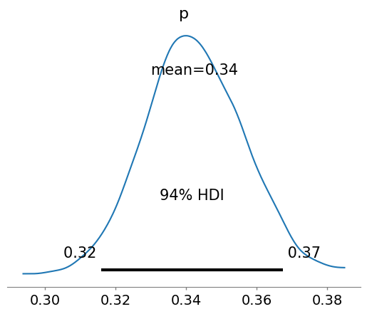
az.plot_posterior(idata, show=True, hdi_prob=0.95)

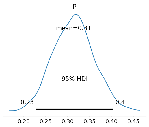
<Axes: title={'center': 'p'}>

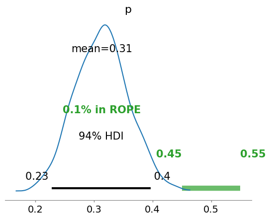
ROPE: Region Of Practical Equivalence#

A range of parameter values around the “null value”, that is good enough for practical purposes link text

# ROPE: Region Of Practical Equivalence
az.plot_posterior(idata, rope=[0.45, .55])

<Axes: title={'center': 'p'}>

Plotting the Posterior#

az.plot_trace(idata, combined = False, compact=False)

array([[<Axes: title={'center': 'p'}>, <Axes: title={'center': 'p'}>]],
      dtype=object)

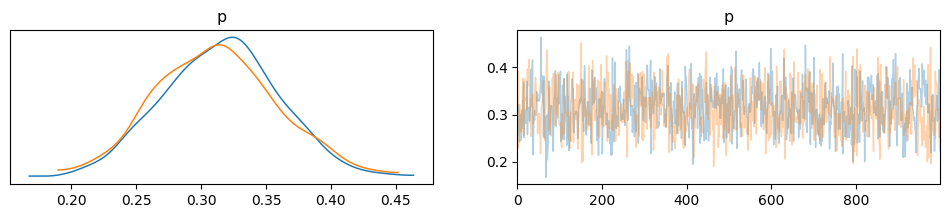
Depending on the number of chains (N), you have N curves.

The plots on the left are obtained from Kernel Density Estimation (KDE) of the corresponding histograms, while the plots on the right are the sampled values from each chain.

You should compare these curves with those obtained analytically in the previous lecture.

Summarizing the Posterior#

#it returns a Pandas dataframe
az.summary(idata)

	mean	sd	hdi_3%	hdi_97%	mcse_mean	mcse_sd	ess_bulk	ess_tail	r_hat
p	0.314	0.046	0.228	0.397	0.002	0.001	924.0	1352.0	1.0

That’s the mean from all the chains… HDI are simple to understand at this point. The other metrics will become more clear in the following lectures, but for now know that they are used to interpret the results of a Bayesian inference.

HPD: High Posterior Density; HDI: is the highest density interval. Another way of summarizing a distribution, which we will use often, abbreviated HDI. The HDI indicates which points of a distribution are most credible, and which cover most of the distribution.

They are often used as synonyms in the legends of the plots.

Geeks If you want to learn more:

mcse: Monte Carlo Standard Error
ess: effective-sample size
ess_bulk: useful measure for sampling efficiency in the bulk of the distribution. The rule of thumb for ess_bulk is for this value to be greater than 100 per chain on average. Since we ran N chains, we need ess_bulk to be greater than N*100 for each parameter.
ess_tail: compute a tail effective sample size estimate for a single variable. The rule of thumb for this value is also to be greater than 100 per chain on average.
r_hat: diagnostic tests for lack of convergence by comparing the variance between multiple chains to the variance within each chain. converges to unity when each of the traces is a sample from the target posterior. Values greater than one indicate that one or more chains have not yet converged.

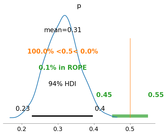
So, is the coin fair? Posterior-based decisions#

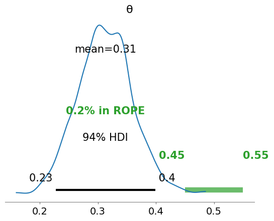
Strictly speaking, a fair coin θ=0.5. But the probability of observing exactly 0.5 is practcally 0. We can relax this definition of fairness to a Region of Practical Equivalence (ROPE), say [0.45,0.55] (it depends on your expectations and prior knowledge and it is always context-dependent).

There are three scenarios:

the ROPE does not overlap with the HDI; the coin is not fair
the ROPE contains the entire HDI; the coin is fair
the ROPE partially overlaps with HDI; we cannot make any conclusions

Unlike a frequentist approach, Bayesian inference is not based on statistical significance, where effects are tested against “zero”. Indeed, the Bayesian framework offers a probabilistic view of the parameters, allowing assessment of the uncertainty related to them. Thus, rather than concluding that an effect is present when it simply differs from zero, we would conclude that the probability of being outside a specific range that can be considered as “practically no effect” (i.e., a negligible magnitude) is sufficient. This range is called the region of practical equivalence (ROPE).

Therefore, the idea underlining ROPE is to let the user define an area around the null value enclosing values that are equivalent to the null value for practical purposes

# you can set reference values if useful for illustrative purposes
az.plot_posterior(idata, ref_val=0.5, rope=[0.45,0.55])

<Axes: title={'center': 'p'}>

Will you get the “same” distribution if you collect and update your beliefs from an array of individual trials?#

indices_to_set = np.random.choice(trials, successes, replace=False)
data_coins = np.zeros(trials, dtype=int)
data_coins[indices_to_set]=1
print(data_coins)
print(np.sum(data_coins))

[1 0 0 0 1 1 1 0 0 1 0 0 1 0 0 0 0 1 1 0 1 1 0 0 0 0 0 0 0 1 1 0 0 1 1 1 0
 0 1 0 0 0 0 0 0 0 1 0 0 1 0 1 1 1 0 0 0 0 0 0 0 0 0 0 1 0 1 1 0 1 0 0 0 1
 1 1 0 0 0 0 0 0 0 1 0 0 0 0 0 0 0 1 0 0 0 1 0 0 0 0]
31

with pm.Model() as model_bernoulli: #everything inside the with-block will add to our_first_model
    # prior
    θ = pm.Beta('θ', alpha=1., beta=1.)
    # likelihood
    y = pm.Bernoulli('y', p=θ, observed=data_coins) #using observed data tells PyMC this is the likelihood

    #"The Inference Button"
    idata_bern = pm.sample()

100.00% [2000/2000 00:00<00:00 Sampling chain 0, 0 divergences]

100.00% [2000/2000 00:00<00:00 Sampling chain 1, 0 divergences]

az.plot_posterior(idata_bern, rope=[0.45, .55])

<Axes: title={'center': 'θ'}>

How to update beliefs with new observations?#

# Extract posterior statistics
posterior_mean_bern = idata_bern.posterior['θ'].mean().values
posterior_sd_bern = idata_bern.posterior['θ'].std().values

print(f"posterior mu: {posterior_mean_bern}, sigma: {posterior_sd_bern}")

# New observations
new_observations = [1, 1]  # For example, two new heads

posterior mu: 0.3128554252365491, sigma: 0.046143176876130114

# Updated model
with pm.Model() as model_updated:
    # Using the posterior mean and sd as new prior
    θ_new = pm.Normal('θ_new', mu=posterior_mean_bern, sigma=posterior_sd_bern)

    # Add new observations to the likelihood
    y_new = pm.Bernoulli('y_new', p=θ_new, observed=new_observations)

    idata_updated = pm.sample()

100.00% [2000/2000 00:00<00:00 Sampling chain 0, 0 divergences]

100.00% [2000/2000 00:00<00:00 Sampling chain 1, 0 divergences]

az.plot_posterior(idata_updated, rope=[0.45, .55])

<Axes: title={'center': 'θ_new'}>

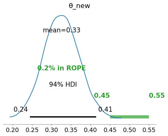
Please notice that the prior we utilized is a normal distrbution, that can give values of the parameter \(\theta\) (a probability) negative. There are ways to “prevent” that, as we will learn in the next lectures.

Similarly, let’s suppose to update the Binomial model with additional information

# Extract posterior statistics
posterior_mean_bin = idata.posterior['p'].mean().values
posterior_sd_bin = idata.posterior['p'].std().values

print(f"posterior mu: {posterior_mean_bin}, sigma: {posterior_sd_bin}")

# New observations
new_heads = 346  # For example, two new heads
new_trials = 1000

tot_trials = trials + new_trials
tot_heads = successes + new_heads

print(f"tot_trials: {tot_trials}, tot_heads: {tot_heads}")
print(f"new_trials: {new_trials}, new_heads: {new_heads}")
print(f"previous trials: {trials}, heads: {successes} ")

posterior mu: 0.3135352187331132, sigma: 0.04556663966440773
tot_trials: 1100, tot_heads: 377
new_trials: 1000, new_heads: 346
previous trials: 100, heads: 31 

with pm.Model() as update_binom:

  p = pm.Normal("p",mu=posterior_mean_bin,sigma = posterior_sd_bin)

  obs = pm.Binomial("obs",n = new_trials, p=p, observed = new_heads)

  idata_bin_update = pm.sample()

100.00% [2000/2000 00:00<00:00 Sampling chain 0, 0 divergences]

100.00% [2000/2000 00:00<00:00 Sampling chain 1, 0 divergences]

az.plot_posterior(idata_bin_update)

<Axes: title={'center': 'p'}>

Again, please notice that the prior we utilized is a normal distrbution, that can give values of the parameter to infer, a probability, negative. There are ways to “prevent” that, as we will learn in the next lectures…

Bayesian Reasoning in Data Science (DATA 644)

Intro to Probabilsitic Programming (PyMC)

Contents

Intro to Probabilsitic Programming (PyMC)#

pymc.sample#

Exploring the model and the obtained chains#

Arviz - Exploratory analysis of Bayesian models#

ROPE: Region Of Practical Equivalence#

Plotting the Posterior#

Summarizing the Posterior#

So, is the coin fair? Posterior-based decisions#

Will you get the “same” distribution if you collect and update your beliefs from an array of individual trials?#

How to update beliefs with new observations?#