Bayesian Linear Regression
Contents
Bayesian Linear Regression#
%pip install pymc pytensor
Requirement already satisfied: pymc in /usr/local/lib/python3.10/dist-packages (5.7.2)
Requirement already satisfied: pytensor in /usr/local/lib/python3.10/dist-packages (2.14.2)
Requirement already satisfied: arviz>=0.13.0 in /usr/local/lib/python3.10/dist-packages (from pymc) (0.15.1)
Requirement already satisfied: cachetools>=4.2.1 in /usr/local/lib/python3.10/dist-packages (from pymc) (5.3.2)
Requirement already satisfied: cloudpickle in /usr/local/lib/python3.10/dist-packages (from pymc) (2.2.1)
Requirement already satisfied: fastprogress>=0.2.0 in /usr/local/lib/python3.10/dist-packages (from pymc) (1.0.3)
Requirement already satisfied: numpy>=1.15.0 in /usr/local/lib/python3.10/dist-packages (from pymc) (1.25.2)
Requirement already satisfied: pandas>=0.24.0 in /usr/local/lib/python3.10/dist-packages (from pymc) (1.5.3)
Requirement already satisfied: scipy>=1.4.1 in /usr/local/lib/python3.10/dist-packages (from pymc) (1.11.4)
Requirement already satisfied: typing-extensions>=3.7.4 in /usr/local/lib/python3.10/dist-packages (from pymc) (4.9.0)
Requirement already satisfied: setuptools>=48.0.0 in /usr/local/lib/python3.10/dist-packages (from pytensor) (67.7.2)
Requirement already satisfied: filelock in /usr/local/lib/python3.10/dist-packages (from pytensor) (3.13.1)
Requirement already satisfied: etuples in /usr/local/lib/python3.10/dist-packages (from pytensor) (0.3.9)
Requirement already satisfied: logical-unification in /usr/local/lib/python3.10/dist-packages (from pytensor) (0.4.6)
Requirement already satisfied: miniKanren in /usr/local/lib/python3.10/dist-packages (from pytensor) (1.0.3)
Requirement already satisfied: cons in /usr/local/lib/python3.10/dist-packages (from pytensor) (0.4.6)
Requirement already satisfied: matplotlib>=3.2 in /usr/local/lib/python3.10/dist-packages (from arviz>=0.13.0->pymc) (3.7.1)
Requirement already satisfied: packaging in /usr/local/lib/python3.10/dist-packages (from arviz>=0.13.0->pymc) (23.2)
Requirement already satisfied: xarray>=0.21.0 in /usr/local/lib/python3.10/dist-packages (from arviz>=0.13.0->pymc) (2023.7.0)
Requirement already satisfied: h5netcdf>=1.0.2 in /usr/local/lib/python3.10/dist-packages (from arviz>=0.13.0->pymc) (1.3.0)
Requirement already satisfied: xarray-einstats>=0.3 in /usr/local/lib/python3.10/dist-packages (from arviz>=0.13.0->pymc) (0.7.0)
Requirement already satisfied: python-dateutil>=2.8.1 in /usr/local/lib/python3.10/dist-packages (from pandas>=0.24.0->pymc) (2.8.2)
Requirement already satisfied: pytz>=2020.1 in /usr/local/lib/python3.10/dist-packages (from pandas>=0.24.0->pymc) (2023.4)
Requirement already satisfied: toolz in /usr/local/lib/python3.10/dist-packages (from logical-unification->pytensor) (0.12.1)
Requirement already satisfied: multipledispatch in /usr/local/lib/python3.10/dist-packages (from logical-unification->pytensor) (1.0.0)
Requirement already satisfied: h5py in /usr/local/lib/python3.10/dist-packages (from h5netcdf>=1.0.2->arviz>=0.13.0->pymc) (3.9.0)
Requirement already satisfied: contourpy>=1.0.1 in /usr/local/lib/python3.10/dist-packages (from matplotlib>=3.2->arviz>=0.13.0->pymc) (1.2.0)
Requirement already satisfied: cycler>=0.10 in /usr/local/lib/python3.10/dist-packages (from matplotlib>=3.2->arviz>=0.13.0->pymc) (0.12.1)
Requirement already satisfied: fonttools>=4.22.0 in /usr/local/lib/python3.10/dist-packages (from matplotlib>=3.2->arviz>=0.13.0->pymc) (4.48.1)
Requirement already satisfied: kiwisolver>=1.0.1 in /usr/local/lib/python3.10/dist-packages (from matplotlib>=3.2->arviz>=0.13.0->pymc) (1.4.5)
Requirement already satisfied: pillow>=6.2.0 in /usr/local/lib/python3.10/dist-packages (from matplotlib>=3.2->arviz>=0.13.0->pymc) (9.4.0)
Requirement already satisfied: pyparsing>=2.3.1 in /usr/local/lib/python3.10/dist-packages (from matplotlib>=3.2->arviz>=0.13.0->pymc) (3.1.1)
Requirement already satisfied: six>=1.5 in /usr/local/lib/python3.10/dist-packages (from python-dateutil>=2.8.1->pandas>=0.24.0->pymc) (1.16.0)
import numpy as np
import pymc as pm
import matplotlib.pyplot as plt
import arviz as az
Exercise: Simple Linear Regression#
np.random.seed(123)

N = 100
x = np.random.normal(10,1,N)
eps = np.random.normal(0,0.5,size=N)

alpha_real = 2.5
beta_real = 0.9

y_real = alpha_real + beta_real*x

y = y_real + eps

print(f"x, {x[: 5]}, ... {x[-2 :]}")
print(f"y, {y[: 5]}, ... {y[-2 :]}")

"""
# what happens if you center your data around the origin?
y = y - np.mean(y)
x = x - np.mean(x)
y_real = y_real - np.mean(y_real)
"""
x, [ 8.9143694  10.99734545 10.2829785   8.49370529  9.42139975], ... [10.37940061  9.62082357]
y, [10.8439598  11.40866694 12.11081297 11.44348672 10.96694678], ... [11.67082969 11.04976808]
'\n# what happens if you center your data around the origin?\ny = y - np.mean(y)\nx = x - np.mean(x)\ny_real = y_real - np.mean(y_real)\n'
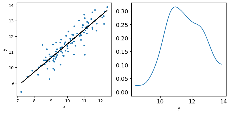
_, ax = plt.subplots(1,2,figsize=(8,4))
ax[0].plot(x,y,'C0.')
ax[0].set_xlabel('x')
ax[0].set_ylabel('y')
ax[0].plot(x,y_real,'k')
az.plot_kde(y,ax=ax[1])
ax[1].set_xlabel('y')
plt.tight_layout()
with pm.Model() as model_lin:
    α = pm.Normal('α', mu=0, sigma=10)
    β = pm.Normal('β', mu=0, sigma=1)
    ϵ = pm.HalfCauchy('ϵ', 5)

    μ = pm.Deterministic('μ', α + β * x)

    # Deterministic nodes are computed outside the main computation graph,
    # which can be optimized as though there was no Deterministic nodes.
    # Whereas the optimized graph can be evaluated thousands of times during a NUTS step,
    # the Deterministic quantities are just computeed once at the end of the step,
    # with the final values of the other random variables

    y_pred = pm.Normal('y_pred', mu=α + β * x, sigma=ϵ, observed=y)

    trace_lin = pm.sample(1000, tune=1000)
100.00% [2000/2000 00:09<00:00 Sampling chain 0, 0 divergences]
100.00% [2000/2000 00:11<00:00 Sampling chain 1, 0 divergences]
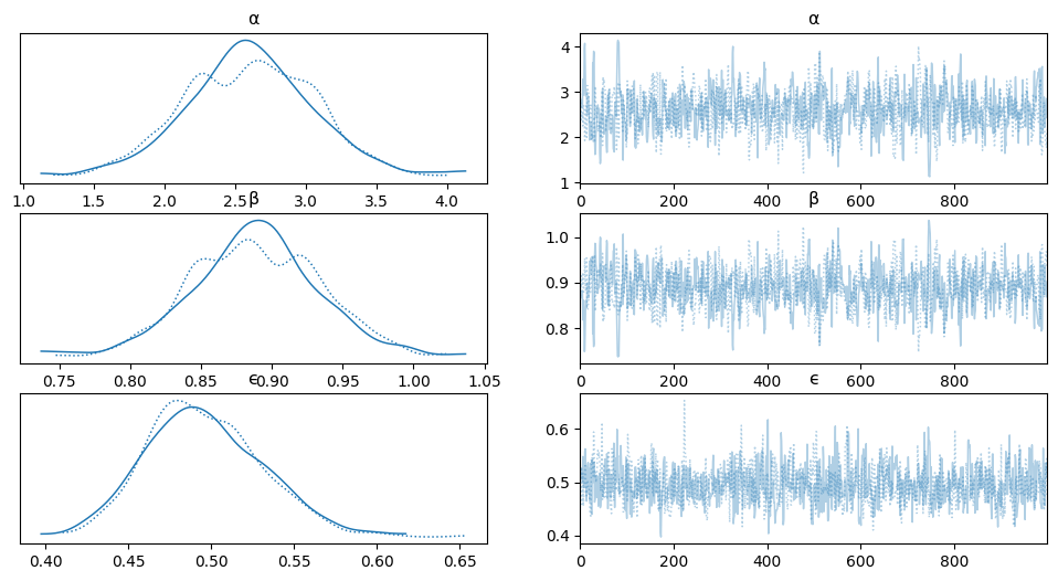
az.plot_trace(trace_lin, var_names=['α', 'β', 'ϵ'])
array([[<Axes: title={'center': 'α'}>, <Axes: title={'center': 'α'}>],
       [<Axes: title={'center': 'β'}>, <Axes: title={'center': 'β'}>],
       [<Axes: title={'center': 'ϵ'}>, <Axes: title={'center': 'ϵ'}>]],
      dtype=object)
az.summary(trace_lin)
| mean | sd | hdi_3% | hdi_97% | mcse_mean | mcse_sd | ess_bulk | ess_tail | r_hat | |
|---|---|---|---|---|---|---|---|---|---|
| α | 2.603 | 0.455 | 1.779 | 3.478 | 0.018 | 0.013 | 671.0 | 576.0 | 1.0 |
| β | 0.889 | 0.045 | 0.802 | 0.970 | 0.002 | 0.001 | 665.0 | 721.0 | 1.0 |
| ϵ | 0.496 | 0.035 | 0.431 | 0.559 | 0.001 | 0.001 | 925.0 | 913.0 | 1.0 |
| μ[0] | 10.526 | 0.071 | 10.395 | 10.658 | 0.002 | 0.002 | 936.0 | 1142.0 | 1.0 |
| μ[1] | 12.377 | 0.064 | 12.263 | 12.503 | 0.002 | 0.001 | 989.0 | 1288.0 | 1.0 |
| ... | ... | ... | ... | ... | ... | ... | ... | ... | ... |
| μ[95] | 12.407 | 0.065 | 12.290 | 12.533 | 0.002 | 0.001 | 972.0 | 1221.0 | 1.0 |
| μ[96] | 10.527 | 0.070 | 10.396 | 10.659 | 0.002 | 0.002 | 937.0 | 1142.0 | 1.0 |
| μ[97] | 10.279 | 0.080 | 10.128 | 10.422 | 0.003 | 0.002 | 860.0 | 1028.0 | 1.0 |
| μ[98] | 11.828 | 0.050 | 11.730 | 11.917 | 0.001 | 0.001 | 1490.0 | 1530.0 | 1.0 |
| μ[99] | 11.153 | 0.052 | 11.065 | 11.260 | 0.001 | 0.001 | 1385.0 | 1434.0 | 1.0 |
103 rows × 9 columns
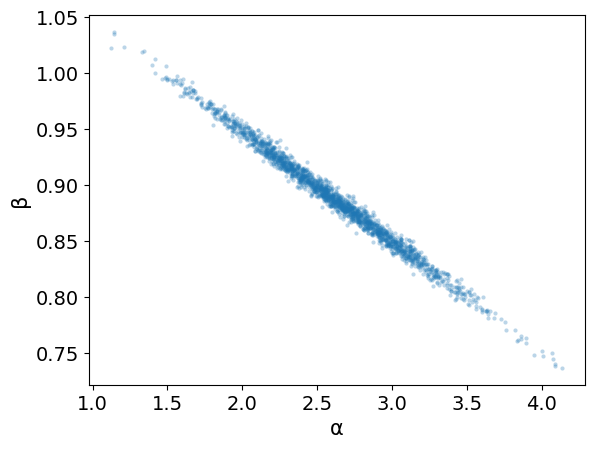
az.plot_pair(trace_lin,var_names=['α','β'], scatter_kwargs={'alpha': 0.3})
<Axes: xlabel='α', ylabel='β'>
res = az.summary(trace_lin) #pandas DataFrame
alpha_m = res.loc['α']['mean']
beta_m = res.loc['β']['mean']
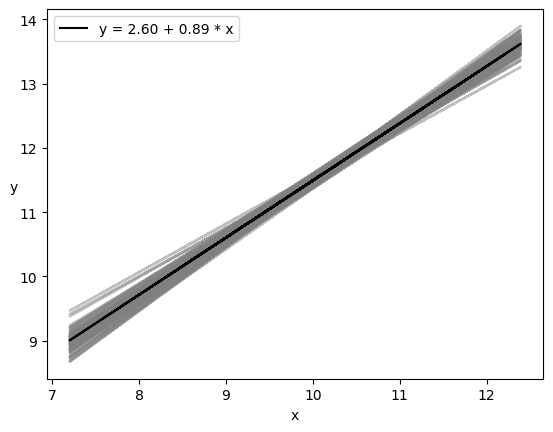
trace_a = trace_lin['posterior']['α'][0].values
trace_b = trace_lin['posterior']['β'][0].values
draws = range(0, len(trace_lin['posterior']['α'][0]), 10)
plt.plot(x, trace_a[draws] + trace_b[draws]
* x[:, np.newaxis], c='gray', alpha=0.5);
plt.plot(x, alpha_m + beta_m * x, c='k',
label=f'y = {alpha_m:.2f} + {beta_m:.2f} * x');
plt.xlabel('x')
plt.ylabel('y', rotation=0)
plt.legend();
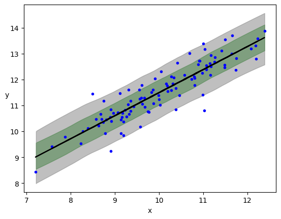
ppc = pm.sample_posterior_predictive(trace_lin, model=model_lin)
100.00% [2000/2000 00:00<00:00]
ppc
arviz.InferenceData
-
<xarray.Dataset> Dimensions: (chain: 2, draw: 1000, y_pred_dim_2: 100) Coordinates: * chain (chain) int64 0 1 * draw (draw) int64 0 1 2 3 4 5 6 7 ... 993 994 995 996 997 998 999 * y_pred_dim_2 (y_pred_dim_2) int64 0 1 2 3 4 5 6 7 ... 93 94 95 96 97 98 99 Data variables: y_pred (chain, draw, y_pred_dim_2) float64 10.94 11.69 ... 12.1 10.29 Attributes: created_at: 2024-02-15T14:50:22.591667 arviz_version: 0.15.1 inference_library: pymc inference_library_version: 5.7.2 -
<xarray.Dataset>
Dimensions:       (y_pred_dim_0: 100)
Coordinates:
  * y_pred_dim_0  (y_pred_dim_0) int64 0 1 2 3 4 5 6 7 ... 93 94 95 96 97 98 99
Data variables:
    y_pred        (y_pred_dim_0) float64 10.84 11.41 12.11 ... 10.22 11.67 11.05
Attributes:
    created_at:                 2024-02-15T14:50:22.594074
    arviz_version:              0.15.1
    inference_library:          pymc
    inference_library_version:  5.7.2
plt.plot(x, y, 'b.')


plt.plot(x, alpha_m + beta_m * x, c='k',
         label=f'y = {alpha_m:.2f} + {beta_m:.2f} * x')


az.plot_hdi(x, ppc.posterior_predictive['y_pred'], hdi_prob=0.68, color='green')
az.plot_hdi(x, ppc.posterior_predictive['y_pred'], hdi_prob=0.95, color='gray')

plt.xlabel('x')
plt.ylabel('y', rotation=0)
Text(0, 0.5, 'y')
Comparison with Ordinary Least Squares#
from scipy import stats
lreg = stats.linregress(x,y)

slope = lreg.slope
slope_err = lreg.stderr
interc = lreg.intercept
interc_err = lreg.intercept_stderr


res = az.summary(trace_lin)
alpha_m = res.loc['α']['mean']
alpha_s = res.loc['α']['sd']
beta_m  = res.loc['β']['mean']
beta_s = res.loc['β']['sd']

print("\nOLS:\nα= {:1.3} +/- {:1.3}".format(interc,interc_err))
print("β= {:1.3} +/- {:1.3}\n".format(slope,slope_err))
print("\nBayesLR:\nα= {:1.3} +/- {:1.3}".format(alpha_m,alpha_s))
print("β= {:1.3} +/- {:1.3}\n".format(beta_m,beta_s))
OLS:
α= 2.57 +/- 0.438
β= 0.892 +/- 0.0434


BayesLR:
α= 2.59 +/- 0.433
β= 0.89 +/- 0.043
Robust Linear Regression#
N = 10
x = np.random.normal(10,1,N)
eps = np.random.normal(0,0.5,size=N)

alpha_real = 2.5
beta_real = 0.9

y = alpha_real + beta_real*x

#Let's add an outlier
x_o = 10.0
y_o = 12.5

# the new dataset
xn = np.append(x,x_o)
yn = np.append(y,y_o)


# centering datasets
x = x-np.mean(x)
y = y-np.mean(y)

xn = xn-np.mean(xn)
yn = yn-np.mean(yn)
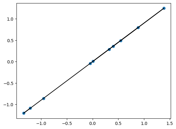
plt.scatter(x,y)
plt.plot(x,y,'k')
[<matplotlib.lines.Line2D at 0x7f766af1d630>]
plt.scatter(xn,yn)
<matplotlib.collections.PathCollection at 0x7f765e259900>
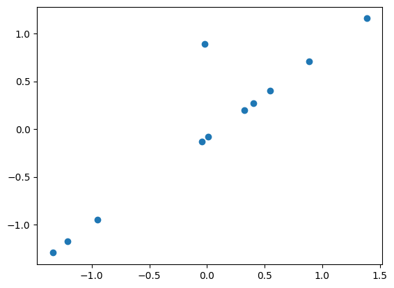
Now if you do a fit, the results of alpha and beta will be affected by the outlier point
lreg = stats.linregress(x,y)

slope = lreg.slope
slope_err = lreg.stderr
interc = lreg.intercept
interc_err = lreg.intercept_stderr

print("\nOLS:\nα= {:1.3} +/- {:1.3}".format(interc,interc_err))
print("β= {:1.3} +/- {:1.3}\n".format(slope,slope_err))
OLS:
α= -4.26e-16 +/- 0.0
β= 0.9 +/- 0.0
lreg = stats.linregress(xn,yn)

slope_n = lreg.slope
slope_err_n = lreg.stderr
interc_n = lreg.intercept
interc_err_n = lreg.intercept_stderr

print("\nOLS:\nα= {:1.3} +/- {:1.3}".format(interc_n,interc_err_n))
print("β= {:1.3} +/- {:1.3}\n".format(slope_n,slope_err_n))
OLS:
α= 1.61e-16 +/- 0.0958
β= 0.898 +/- 0.117
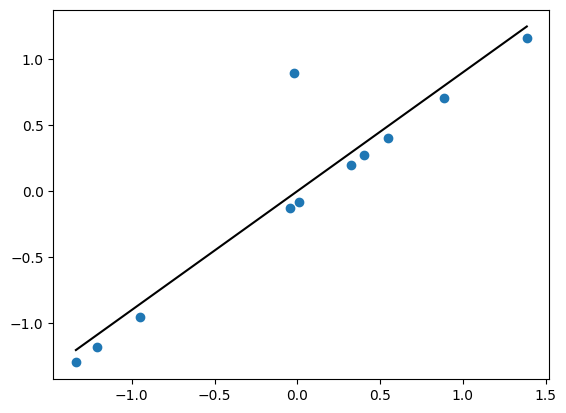
plt.scatter(xn,yn)

xp = np.linspace(np.min(xn),np.max(xn),100)

yp = interc_n + slope_n*xp

plt.plot(xp,yp,'k-')
[<matplotlib.lines.Line2D at 0x7f765e240df0>]
with pm.Model() as model_t:
    α = pm.Normal('α', mu=0, sigma=0.2)
    β = pm.Normal('β', mu=0, sigma=1)
    #ϵ = pm.HalfNormal('ϵ', 3)
    ν_ = pm.Exponential('ν_', 1/29)
    ν = pm.Deterministic('ν', ν_ + 1) #a shifted exponential to avoid values of ν close to 0

    y_pred = pm.StudentT('y_pred', mu=α + β * xn,
                         sigma=0.1, nu=ν, observed=yn) #ϵ

    trace_t = pm.sample(2000, tune=1000, return_inferencedata=True)
100.00% [3000/3000 00:03<00:00 Sampling chain 0, 0 divergences]
100.00% [3000/3000 00:03<00:00 Sampling chain 1, 0 divergences]
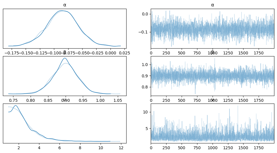
varnames = ['α', 'β', 'ν']
az.plot_trace(trace_t, var_names=varnames);
rest = az.summary(trace_t)
alpha_m = rest.loc['α']['mean']
beta_m = rest.loc['β']['mean']
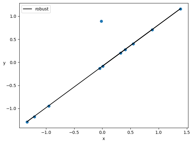
plt.plot(xn, alpha_m + beta_m * xn, c='k', label='robust')
plt.scatter(xn,yn)
plt.xlabel('x')
plt.ylabel('y', rotation=0)
plt.legend(loc=2)
plt.tight_layout()