
Thinking Probabilistically (mod1-part1)
Contents
Thinking Probabilistically (mod1-part1)#
Coin Flipping Problem#
\(\theta\) is the bias in the coin flipping problem: if it is a fair coin you’d get 0.5; you want to infer the actual bias from observations.
You toss the coin N times. Let’s define with \(y\) the number of occurrences of heads, and \(\theta\) be the (true) probability of getting a head from the coin.
The following is a binomial distribution:
We will use scipy.stats.binom for the binomial distribution.
Other references
Binomial#
import numpy as np
import matplotlib.pyplot as plt
from scipy import stats
import arviz as az
az.style.use('arviz-darkgrid') #beautify plots with dark grid background and font size
n_params = [1, 2, 4, 6]  # Number of trials
p_params = [0.25, 0.5, 0.75]  # Probability of success (e.g., getting head)

x = np.arange(0, max(n_params)+1)


_,ax = plt.subplots(len(n_params), len(p_params), sharex=True, sharey=True,
                    figsize=(8, 7), constrained_layout=True)

for i in range(len(n_params)):
    for j in range(len(p_params)):
        n = n_params[i]
        p = p_params[j]

        y = stats.binom(n=n, p=p).pmf(x)
        #y = stats.binom.pmf(x,n=n,p=p) # can be also written

        ax[i,j].vlines(x, 0, y, colors='C0', lw=5)
        ax[i,j].set_ylim(0, 1)
        ax[i,j].plot(0, 0, label="N = {:3.2f}\nθ = {:3.2f}".format(n,p), alpha=0)
        ax[i,j].legend()


ax[2,1].set_xlabel('y')
ax[1,0].set_ylabel('p(y | θ, N)')
ax[0,0].set_xticks(x)


#plt.savefig('./output/B11197_01_03.png', dpi=400)
[<matplotlib.axis.XTick at 0x792c20f83b20>,
 <matplotlib.axis.XTick at 0x792c20f83af0>,
 <matplotlib.axis.XTick at 0x792c20f83a00>,
 <matplotlib.axis.XTick at 0x792c20abdfc0>,
 <matplotlib.axis.XTick at 0x792c20ae8910>,
 <matplotlib.axis.XTick at 0x792c20abc430>,
 <matplotlib.axis.XTick at 0x792c20ae9720>]
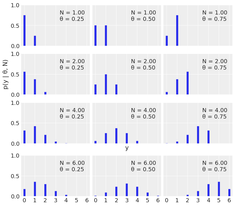
Notice that for discrete distributions, the sum of the heights correspond to actual probabilities.
A Binomial distribution for this problem is a reasonable choice for the likelihood. If we know the value of θ, we can calculate the expected distribution of heads.
The problem is that you may not know the true value of θ (for example, if the coin is not fair)! But here comes the Bayesian reasoning approach: any time you do not know the value of a parameter, we put a prior on it.
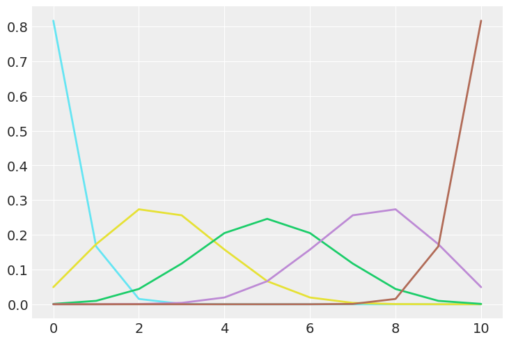
What happens to a posterior if your prior is a Dirac delta distribution? (notice the space of $\theta$ is continuous.)
n=10
p=np.linspace(0.02,0.98,5)

plt.figure()
for i,valp in enumerate(p):

    tstr = 'C'+str(i+5)
    x=np.arange(0,n+1)
    y=stats.binom.pmf(x, n, valp)

    #fig, ax = plt.subplots()

    plt.plot(x, y, linewidth=2.0,color=tstr)
Choosing the Prior#
params = [0.5, 1, 2, 3]
x = np.linspace(0, 1, 100)
f, ax = plt.subplots(len(params), len(params), sharex=True, sharey=True,
                     figsize=(8, 7), constrained_layout=True)
for i in range(4):
    for j in range(4):
        a = params[i]
        b = params[j]
        y = stats.beta(a, b).pdf(x)
        ax[i,j].plot(x, y)
        ax[i,j].plot(0, 0, label="α = {:2.1f}\nβ = {:2.1f}".format(a, b), alpha=0)
        ax[i,j].legend()
ax[1,0].set_yticks([])
ax[3,0].set_xticks([0, 0.5, 1])
f.text(0.5, -0.05, 'θ', ha='center', size=16)
f.text(-0.07, 0.5, 'p(θ)', va='center', rotation=90, size=16)
#plt.savefig('./output/B11197_01_04.png', dpi=400)
Text(-0.07, 0.5, 'p(θ)')
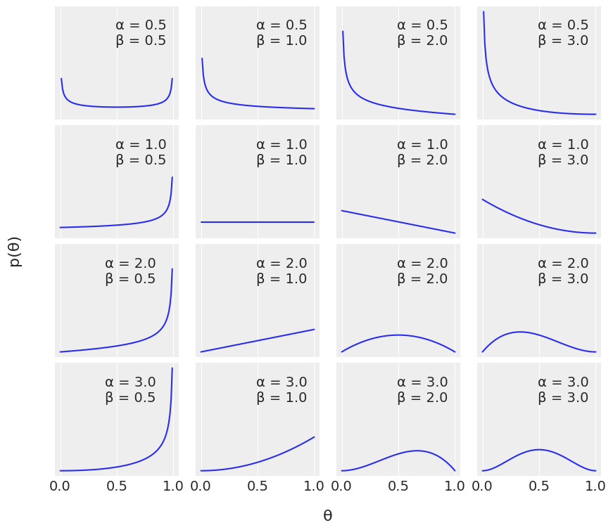
The beta distribution is continuous.
In Bayesian probability theory, if the posterior distribution p(θ | x) is in the same probability distribution family as the prior probability distribution p(θ), the prior and posterior are then called conjugate distributions, and the prior is called a conjugate prior for the likelihood function p(x | θ).
Computing and plotting the posterior#
Now, you must know that the beta distribution looks as follows
\(p(\theta) = \frac{\Gamma(\alpha+\beta)}{\Gamma(\alpha)\Gamma(\beta)}\theta^{\alpha-1}(1-\theta)^{\beta-1}\) (1)
Where \(\Gamma\) is the gamma function. If the maths starts sounding complicated, do not worry. I want you to pay attention to some approximation we can do to calculate the posterior starting from our \(\beta\) prior and our Binomial-likelihood. Later, we will do this calculation more accurately with PyMC, but for now, let’s notice the following:
(1), the \(\beta\)-distribution, looks like a Binomial, with the exception of some factors
From the Bayes’theorem, we know that the posterior is proportional to the likelihood times the prior. Let’s now do the following approximation (remember, \(y\) are the observations):
\(p(\theta|y) \propto \frac{N!}{y!(N-y)!}\theta^{y}(1-\theta)^{N-y} \cdot \frac{\Gamma(\alpha+\beta)}{\Gamma(\alpha)\Gamma(\beta)}\theta^{\alpha-1}(1-\theta)^{\beta-1}\)
Let’s drop all the terms that do not depend on \(\theta\), to get:
\(p(\theta|y) \propto \theta^{y}(1-\theta)^{N-y} \theta^{\alpha-1}(1-\theta)^{\beta-1}\)
that is:
\(p(\theta|y) \propto \theta^{y+\alpha-1}(1-\theta)^{N-y+\beta-1}\)
In other words, the posterior is proportional to a beta-function
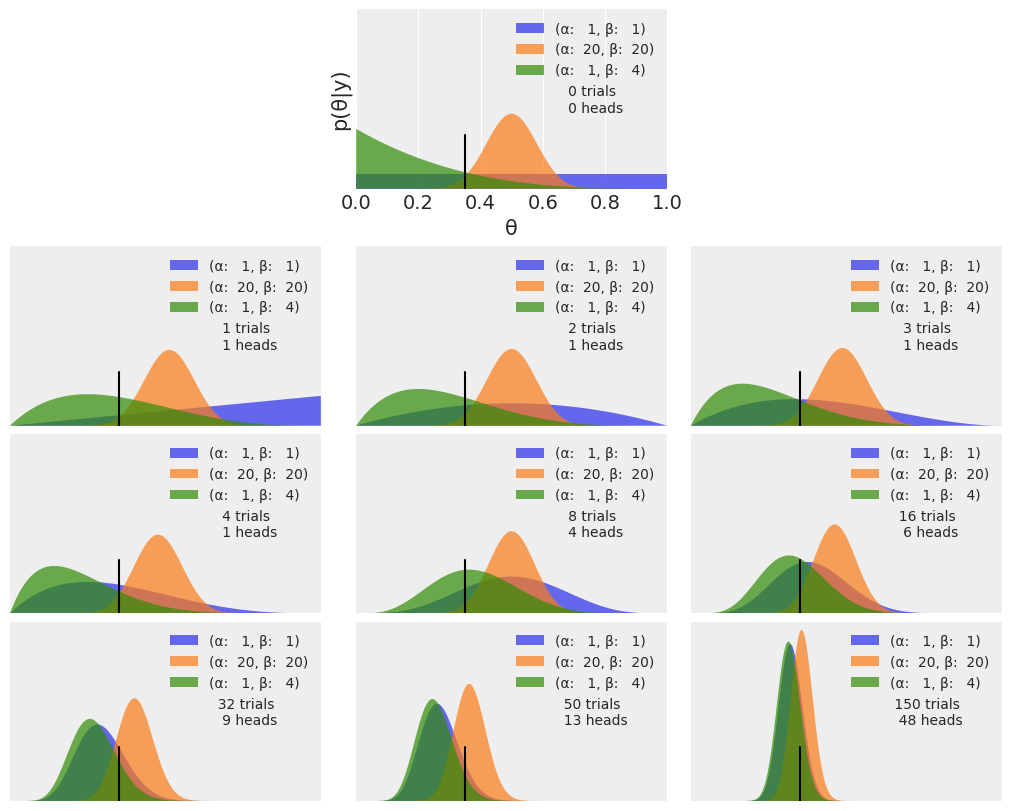
\(p(\theta|y) \propto Beta(\alpha_{prior}+y,\beta_{prior}+N-y)\)
Using the above equation:#
plt.figure(figsize=(10, 8))

n_trials = [0, 1, 2, 3, 4, 8, 16, 32, 50, 150]
data     = [0, 1, 1, 1, 1, 4,  6,  9, 13,  48]
theta_real = 0.35

#------ replace with actual generation from binomial with theta_real ------#
rep_data = []
for nn in n_trials:
    rep_data.append(stats.binom.rvs(nn, theta_real))  #rvs: random variates
#--------------------------------------------------------------------------#

#data = rep_data

beta_params = [(1, 1), (20, 20), (1, 4)]

dist = stats.beta
#https://docs.scipy.org/doc/scipy/reference/generated/scipy.stats.beta.html

x = np.linspace(0, 1, 200)

colors = plt.rcParams["axes.prop_cycle"].by_key()["color"]

for idx, N in enumerate(n_trials):
    if idx == 0:
        plt.subplot(4, 3, 2) #take idx=2 plot
        plt.xlabel('θ')
        plt.ylabel('p(θ|y)')
    else:
        plt.subplot(4, 3, idx+3)
        plt.xticks([])
    y = data[idx]
    for idx2, (a_prior, b_prior) in enumerate(beta_params):
        #tmp_color = colors[idx2]
        p_theta_given_y = dist.pdf(x, a_prior + y, b_prior + N - y)
        plt.fill_between(x, 0, p_theta_given_y,alpha=0.7,
                         label=f'(α: {a_prior:3d}, β: {b_prior:3d})')


    plt.axvline(theta_real, ymax=0.3, color='k')
    plt.plot(0, 0, label=f'{N:4d} trials\n{y:4d} heads', alpha=0)
    plt.xlim(0, 1)
    plt.ylim(0, 12)
    plt.legend(fontsize=10)
    plt.yticks([])


#plt.tight_layout() #check compatibility
#plt.savefig('./output/B11197_01_05.png', dpi=300)
- PMF uses discrete random variables. PDF uses continuous random variables.
- In the first row we have 0 trials, therefore the three curves are our priors for different settings of the beta-distribution parameters
- The most probable value is given by th emode of the posterior
- The spread of the posterior is proportional to the uncertainty about the value of a parameter
- Given a sufficiently large amount of data, Bayesian models with different priors converge to the same result!
- How fast posteriors converge depend on the data and the model
- It can be demonstrated that the same result is obtained by updating the posterior sequentially than if we do it all at once
- Priors can influence inference... some peoplelike the idea of flat, weakly informative priors
- we have seen though prior information can be essential in some cases, e.g., if the parameter has to be positive
- Priors can make our models work better.
- Frequentist approach estimates parameters through maximum likelihood, avoiding setting up a prior, and works by findining the value of θ that maximizes the likelihood. We have seen in our exercises the limitations of this approach.