Reference:

• Sebastian Raschka, Yuxi Hayden Liu, and Vahid Mirjalili. Machine Learning with PyTorch and Scikit-Learn: Develop machine learning and deep learning models with Python. Packt Publishing Ltd, 2022.

6. Adaline (Adaptive Linear Neuron)

from IPython.display import Image
from IPython.display import display

display(Image(url="https://raw.githubusercontent.com/cfteach/NNDL_DATA621/webpage-src/DATA621/DATA621/images/adaline_flowchart.png", width=700))

import numpy as np


class Adaline:
    """Perceptron classifier.

    Parameters
    ------------
    eta : float
      Learning rate (between 0.0 and 1.0)
    n_iter : int
      Passes over the training dataset.
    random_state : int
      Random number generator seed for random weight
      initialization.

    Attributes
    -----------
    w_ : 1d-array
      Weights after fitting.
    b_ : Scalar
      Bias unit after fitting.
    losses_ : list
      Mean squared error loss values at each epoch

    """
    def __init__(self, eta=0.01, n_iter=50, random_state=1):
        self.eta = eta
        self.n_iter = n_iter
        self.random_state = random_state

    def fit(self, X, y):
        """Fit training data.

        Parameters
        ----------
        X : {array-like}, shape = [n_examples, n_features]
          Training vectors, where n_examples is the number of examples and
          n_features is the number of features.
        y : array-like, shape = [n_examples]
          Target values.

        Returns
        -------
        self : object

        """
        rgen = np.random.RandomState(self.random_state)
        self.w_ = rgen.normal(loc=0.0, scale=0.01, size=X.shape[1])
        self.b_ = np.float_(0.)

        self.losses_ = []

        for i in range(self.n_iter):
          net_input = self.net_input(X)
          output = self.activation(net_input)
          errors = (y-output)
          # the following is vectorized
          self.w_ += self.eta * 2.0 * X.T.dot(errors) / X.shape[0] #[n_features,n_examples]*[n_examples] = [n_features]
          self.b_ += self.eta * 2.0 * errors.mean()
          loss = (errors**2).mean()
          self.losses_.append(loss)
        return self

    def net_input(self, X):
        """Calculate net input"""
        return np.dot(X, self.w_) + self.b_

    def activation(self, X):
        """Compute linear activation"""
        return X

    def predict(self, X):
        """Return class label after unit step"""
        return np.where(self.activation(self.net_input(X)) >= 0.5, 1, 0)

6.1. Using the Iris data

import os
import pandas as pd

try:
    s = 'https://archive.ics.uci.edu/ml/machine-learning-databases/iris/iris.data'
    print('From URL:', s)
    df = pd.read_csv(s,
                     header=None,
                     encoding='utf-8')

except HTTPError:
    s = 'iris.data'
    print('From local Iris path:', s)
    df = pd.read_csv(s,
                     header=None,
                     encoding='utf-8')

df.tail()

From URL: https://archive.ics.uci.edu/ml/machine-learning-databases/iris/iris.data

	0	1	2	3	4
145	6.7	3.0	5.2	2.3	Iris-virginica
146	6.3	2.5	5.0	1.9	Iris-virginica
147	6.5	3.0	5.2	2.0	Iris-virginica
148	6.2	3.4	5.4	2.3	Iris-virginica
149	5.9	3.0	5.1	1.8	Iris-virginica

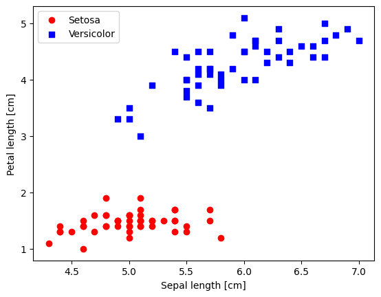
6.2. Plotting the Iris data

%matplotlib inline
import matplotlib.pyplot as plt
import numpy as np



# select setosa and versicolor
#y = df.iloc[0:100, 4].values

y = df.iloc[:, 4].values
X = df.iloc[:, [0, 2]].values  # extract sepal length and petal length

# Map y values to 0, 1, or -1
y_mapped = np.select(
    [y == 'Iris-setosa', y == 'Iris-versicolor'],  # Conditions
    [0, 1],                                        # Values to assign if the condition is True
    default=-1                                     # Value to assign if none of the conditions are True
)


mask = (y_mapped == 0) | (y_mapped == 1)  # Mask for selecting only 0 and 1 in y_mapped


X_filtered = X[mask]
y_filtered = y_mapped[mask]


# Filter the first 50 occurrences of category 0
mask_0 = (y_filtered == 0)
X_0 = X_filtered[mask_0][:50]

# Filter the first 50 occurrences of category 1
mask_1 = (y_filtered == 1)
X_1 = X_filtered[mask_1][:50]


print(np.shape(X_0))
print(np.shape(X_1))


# plot data
plt.scatter(X_0[:, 0], X_0[:, 1],
            color='red', marker='o', label='Setosa')
plt.scatter(X_1[:, 0], X_1[:, 1],
            color='blue', marker='s', label='Versicolor')

plt.xlabel('Sepal length [cm]')
plt.ylabel('Petal length [cm]')
plt.legend(loc='upper left')

(50, 2)
(50, 2)

<matplotlib.legend.Legend at 0x7fe443663100>

6.3. Training the Adaline model

fig, ax = plt.subplots(nrows=1, ncols=2, figsize=(10, 4))

ada1 = Adaline(n_iter=15, eta=0.1).fit(X_filtered, y_filtered)
ax[0].plot(range(1, len(ada1.losses_) + 1), np.log10(ada1.losses_), marker='o')
ax[0].set_xlabel('Epochs')
ax[0].set_ylabel('log(Mean squared error)')
ax[0].set_title('Adaline - Learning rate 0.1')

ada2 = Adaline(n_iter=15, eta=0.0001).fit(X_filtered, y_filtered)
ax[1].plot(range(1, len(ada2.losses_) + 1), ada2.losses_, marker='o')
ax[1].set_xlabel('Epochs')
ax[1].set_ylabel('Mean squared error')
ax[1].set_title('Adaline - Learning rate 0.0001')

plt.show()

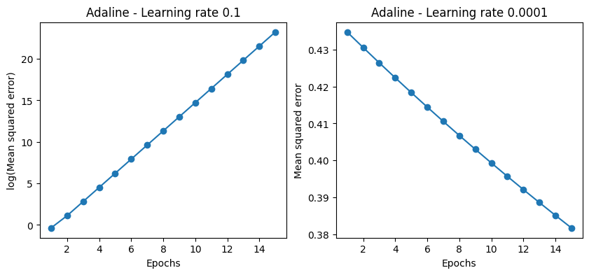
Plot on the left shows that the learning rate is too high, the one on the right that the learning rate is too low.

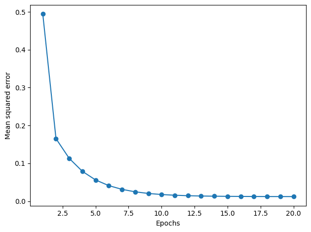
6.4. Standardize Data

This can be very helpful: gradient descent is one of many algorithms that benefit from feature scaling.

X_std = np.copy(X_filtered)
X_std[:,0] = (X_filtered[:,0]-X_filtered[:,0].mean())/X_filtered[:,0].std()
X_std[:,1] = (X_filtered[:,1]-X_filtered[:,1].mean())/X_filtered[:,1].std()

ada_gd = Adaline(n_iter=20, eta=0.5).fit(X_std, y_filtered)

plt.plot(range(1, len(ada_gd.losses_) + 1), ada_gd.losses_, marker='o')
plt.xlabel('Epochs')
plt.ylabel('Mean squared error')

plt.tight_layout()
plt.show()

6.5. Plotting decision regions

from matplotlib.colors import ListedColormap


def plot_decision_regions(X, y, classifier, resolution=0.02):

    # setup marker generator and color map
    markers = ('o', 's', '^', 'v', '<')
    colors = ('red', 'blue', 'lightgreen', 'gray', 'cyan')
    cmap = ListedColormap(colors[:len(np.unique(y))])

    # plot the decision surface
    x1_min, x1_max = X[:, 0].min() - 1, X[:, 0].max() + 1
    x2_min, x2_max = X[:, 1].min() - 1, X[:, 1].max() + 1
    xx1, xx2 = np.meshgrid(np.arange(x1_min, x1_max, resolution),
                           np.arange(x2_min, x2_max, resolution))
    lab = classifier.predict(np.array([xx1.ravel(), xx2.ravel()]).T)
    lab = lab.reshape(xx1.shape)
    plt.contourf(xx1, xx2, lab, alpha=0.3, cmap=cmap)
    plt.xlim(xx1.min(), xx1.max())
    plt.ylim(xx2.min(), xx2.max())

    # plot class examples
    for idx, cl in enumerate(np.unique(y)):
        plt.scatter(x=X[y == cl, 0],
                    y=X[y == cl, 1],
                    alpha=0.8,
                    c=colors[idx],
                    marker=markers[idx],
                    label=f'Class {cl}',
                    edgecolor='black')

plot_decision_regions(X_std, y_filtered, classifier=ada_gd)
plt.xlabel('Sepal length [cm]')
plt.ylabel('Petal length [cm]')
plt.legend(loc='upper left')


plt.show()

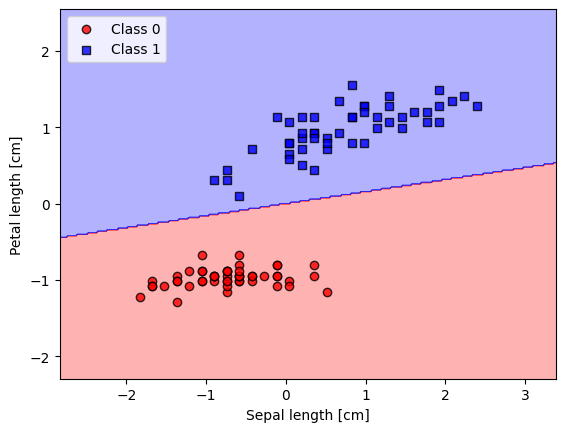
6.6. Accuracy

y_pred = ada_gd.predict(X_std)

accuracy = np.sum(y_pred == y_filtered) / len(y_filtered)
print(f"Accuracy: {accuracy * 100:.2f}%")

Accuracy: 100.00%