Covariance and Kernel

#!pip install pymc3

def exp_quad_kernel(x,knots,l=1):
  return np.array([np.exp(-(x-k)**2/(2*l**2)) for k in knots])

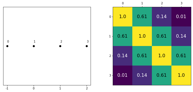
data = np.array([-1,0,1,2])
#data = np.array([-1,0])
cov = exp_quad_kernel(data,data,1)

print(cov)

[[1.         0.60653066 0.13533528 0.011109  ]
 [0.60653066 1.         0.60653066 0.13533528]
 [0.13533528 0.60653066 1.         0.60653066]
 [0.011109   0.13533528 0.60653066 1.        ]]

_, ax=plt.subplots(1,2,figsize=(12,5))

ax[0].plot(data, np.zeros_like(data),'ko')
ax[0].set_yticks([])

for idx,i in enumerate(data):
  ax[0].text(i,0+0.005, idx)
ax[0].set_xticks(data)
ax[0].set_xticklabels(np.round(data,2))

ax[1].grid(False)
im = ax[1].imshow(cov)
colors=['w','k']

for i in range(len(cov)):
  for j in range(len(cov)):
    ax[1].text(i,j, round(cov[i,j],2), color=colors[int(im.norm(cov[i,j])>0.5)], ha = 'center', va='center', fontdict={'size':16})

ax[1].set_xticks(range(len(data)))
ax[1].set_yticks(range(len(data)))
ax[1].xaxis.tick_top()

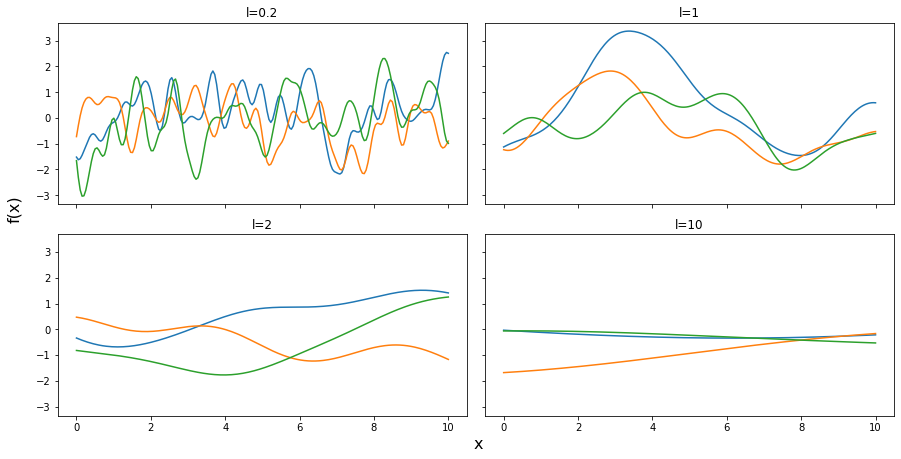
from scipy import stats
np.random.seed(24)
test_points = np.linspace(0,10,200)
fig, ax = plt.subplots(2,2,figsize=(12,6),sharex=True,sharey=True,constrained_layout=True)
ax = np.ravel(ax)
for idx, l in enumerate((0.2,1,2,10)):
  cov = exp_quad_kernel(test_points, test_points, l)
  ax[idx].plot(test_points, stats.multivariate_normal.rvs(cov=cov,size=3).T)
  ax[idx].set_title(f'l={l}')

fig.text(0.51,-0.03,'x', fontsize=16)
fig.text(-0.03,0.5,'f(x)', fontsize=16, rotation=90)

Text(-0.03, 0.5, 'f(x)')

Gaussian Processes

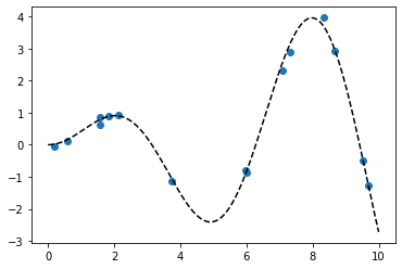
np.random.seed(42)

x = np.random.uniform(0,10,size=15)

scale = 0.50
y = np.random.normal(scale*x*np.sin(x), 0.1)

plt.plot(x,y,'o')

true_x = np.linspace(0,10,200)
true_y = scale*true_x*np.sin(true_x)
plt.plot(true_x,true_y, 'k--')

[<matplotlib.lines.Line2D at 0x7f7a6af02e50>]

X = x[:,None]

import pymc3 as pm

with pm.Model() as model_reg:
  #hyperprior for lengthscale kernel parameter 
  l = pm.Gamma('l',2,0.5)
  #instantiate a covariance function 
  cov = pm.gp.cov.ExpQuad(1,ls=l)
  #mean = pm.gp.mean.Constant(c=0)
  #instantiate a GP prior 
  gp = pm.gp.Marginal(cov_func=cov)#mean_func=mean,
  #prior 
  eps = pm.HalfNormal('eps',25)
  #likelihood 
  y_pred = gp.marginal_likelihood('y_pred',X=X, y=y, noise=eps)
  trace_reg = pm.sample(2000, return_inferencedata=True, target_accept=0.95)

100.00% [3000/3000 00:16<00:00 Sampling chain 0, 0 divergences]

100.00% [3000/3000 00:16<00:00 Sampling chain 1, 0 divergences]

import arviz as az
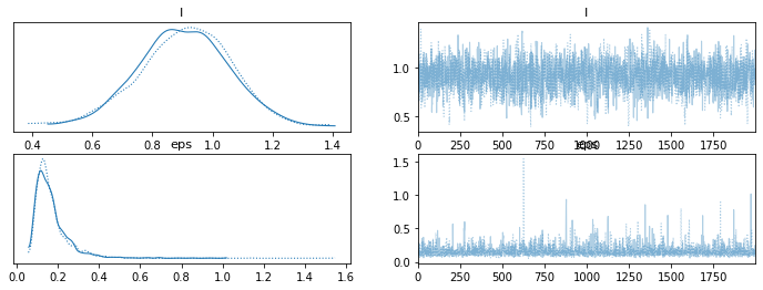
az.plot_trace(trace_reg)

array([[<matplotlib.axes._subplots.AxesSubplot object at 0x7f7a7ce53e90>,
        <matplotlib.axes._subplots.AxesSubplot object at 0x7f7a7e064150>],
       [<matplotlib.axes._subplots.AxesSubplot object at 0x7f7a81c81210>,
        <matplotlib.axes._subplots.AxesSubplot object at 0x7f7a852ab390>]],
      dtype=object)

X_new = np.linspace(np.floor(x.min()), np.ceil(x.max()), 100)[:,None]

with model_reg:
    #del marginal_gp_model.named_vars['f_pred']
    #marginal_gp_model.vars.remove(f_pred)
    f_pred = gp.conditional('f_pred', X_new)

with model_reg:
    pred_samples = pm.sample_posterior_predictive(trace_reg, var_names=['f_pred'], samples=150)

/usr/local/lib/python3.7/dist-packages/pymc3/sampling.py:1709: UserWarning: samples parameter is smaller than nchains times ndraws, some draws and/or chains may not be represented in the returned posterior predictive sample
  "samples parameter is smaller than nchains times ndraws, some draws "

100.00% [150/150 00:03<00:00]

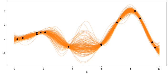
_, ax = plt.subplots(figsize=(12,5))
ax.plot(X_new, pred_samples['f_pred'].T, 'C1-', alpha=0.3)
ax.plot(X, y, 'ko')
ax.set_xlabel('X')

Text(0.5, 0, 'X')

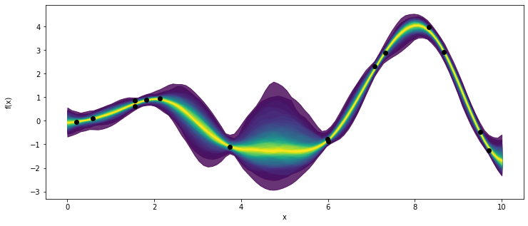
_, ax = plt.subplots(figsize=(12,5))
pm.gp.util.plot_gp_dist(ax,pred_samples['f_pred'], X_new, palette='viridis',plot_samples=False)

ax.plot(X,y,'ko')
ax.set_xlabel('x')
ax.set_ylabel('f(x)',labelpad=25)

Text(0, 0.5, 'f(x)')

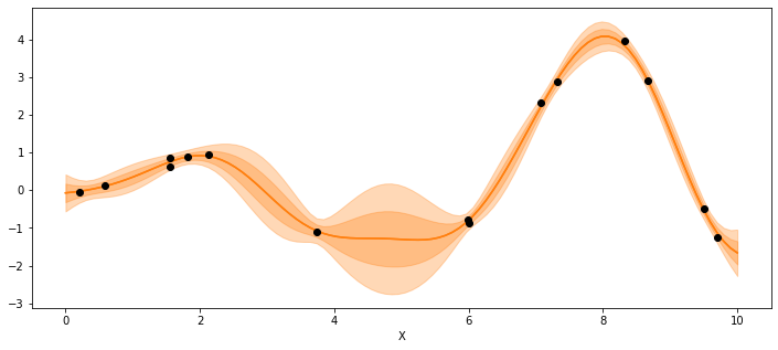
_, ax = plt.subplots(figsize=(12,5))
point = {'l':trace_reg.posterior['l'].mean(), 'eps':trace_reg.posterior['eps'].mean()}

mu, var = gp.predict(X_new,point=point,diag=True)
sd = var**0.5

ax.plot(X_new,mu,'C1')
ax.fill_between(X_new.flatten(),mu-sd,mu+sd, color="C1",alpha=0.3)

ax.plot(X_new,mu,'C1')
ax.fill_between(X_new.flatten(),mu-2*sd,mu+2*sd, color="C1",alpha=0.3)

ax.plot(X,y,'ko')
ax.set_xlabel('X')

Text(0.5, 0, 'X')

Real-world example: Spawning Salmon

credits: https://github.com/fonnesbeck/gp_tutorial_pydata

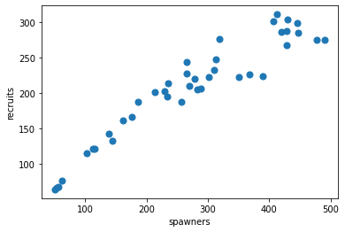
The plot below shows the relationship between the number of spawning salmon in a particular stream and the number of fry that are recruited into the population in the spring.

Biological knowledge suggests this relationship is not linear and we would like to model it.

import requests
import pandas as pd
import io

target_url = 'https://raw.githubusercontent.com/cfteach/brds/main/datasets/salmon.txt'
download = requests.get(target_url).content

salmon_data = pd.read_table(io.StringIO(download.decode('utf-8')), sep='\s+', index_col=0)
salmon_data.plot.scatter(x='spawners', y='recruits', s=50);

#we have prior knowledge about fish population growth, and we can include a linear mean function as a prior

with pm.Model() as salmon_model:

    # Lengthscale
    ρ = pm.HalfCauchy('ρ', 1)
    η = pm.HalfCauchy('η', 1)
    #η=1
    
    M = pm.gp.mean.Linear(coeffs=(salmon_data.recruits/salmon_data.spawners).mean())
    K = (η**2) * pm.gp.cov.ExpQuad(1, ρ) 

with salmon_model:
    
    σ = pm.HalfCauchy('σ', 1)
    
    recruit_gp = pm.gp.Marginal(mean_func=M, cov_func=K)
    recruit_gp.marginal_likelihood('recruits', X=salmon_data.spawners.values.reshape(-1,1), 
                           y=salmon_data.recruits.values, noise=σ)

with salmon_model:
    salmon_trace = pm.sample(1000, return_inferencedata=True)

100.00% [2000/2000 00:22<00:00 Sampling chain 0, 0 divergences]

100.00% [2000/2000 00:16<00:00 Sampling chain 1, 0 divergences]

ERROR:pymc3:The estimated number of effective samples is smaller than 200 for some parameters.

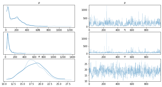
az.plot_trace(salmon_trace, var_names=['ρ','η','σ']) #'η'

array([[<matplotlib.axes._subplots.AxesSubplot object at 0x7f7a651d7150>,
        <matplotlib.axes._subplots.AxesSubplot object at 0x7f7a6606e650>],
       [<matplotlib.axes._subplots.AxesSubplot object at 0x7f7a661a4250>,
        <matplotlib.axes._subplots.AxesSubplot object at 0x7f7a6612ec10>],
       [<matplotlib.axes._subplots.AxesSubplot object at 0x7f7a66299b90>,
        <matplotlib.axes._subplots.AxesSubplot object at 0x7f7a662cf0d0>]],
      dtype=object)

X_pred = np.linspace(0, 500, 100).reshape(-1, 1)

with salmon_model:
    salmon_pred3 = recruit_gp.conditional('salmon_pred3', X_pred)

with salmon_model:
    salmon_samples = pm.sample_posterior_predictive(salmon_trace, var_names=['salmon_pred3'], samples=150)

/usr/local/lib/python3.7/dist-packages/pymc3/sampling.py:1709: UserWarning: samples parameter is smaller than nchains times ndraws, some draws and/or chains may not be represented in the returned posterior predictive sample
  "samples parameter is smaller than nchains times ndraws, some draws "

100.00% [150/150 00:04<00:00]

salmon_data['spawners'].values

array([ 56,  62, 445, 279, 138, 428, 319, 102,  51, 289, 351, 282, 310,
       266, 256, 144, 447, 186, 389, 113, 412, 176, 313, 162, 368,  54,
       214, 429, 115, 407, 265, 301, 234, 229, 270, 478, 419, 490, 430,
       235])

_, ax = plt.subplots(figsize=(12,5))
ax.plot(X_pred, salmon_samples['salmon_pred3'].T, 'C1-', alpha=0.3)
ax.plot(salmon_data['spawners'].values,salmon_data['recruits'].values, 'ko')
#ax.set_xlabel('X')

[<matplotlib.lines.Line2D at 0x7f7a63ec4410>]

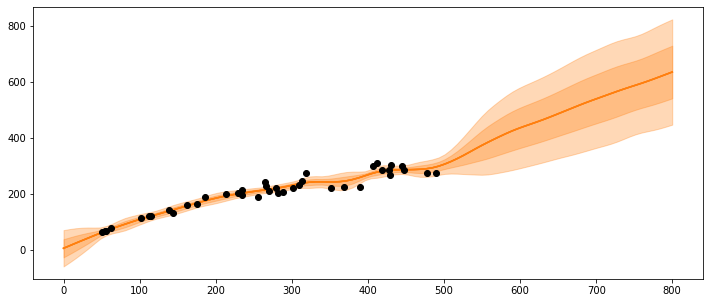
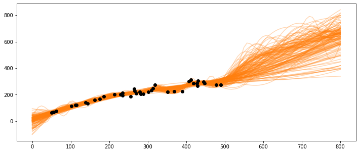
What happens if the population gets very large, e.g., at 600 or 800 spawners?

X_pred = np.linspace(0, 800, 100).reshape(-1, 1)

with salmon_model:
    salmon_pred4 = recruit_gp.conditional('salmon_pred4', X_pred)

with salmon_model:
    salmon_samples = pm.sample_posterior_predictive(salmon_trace, var_names=['salmon_pred4'], samples=150)

/usr/local/lib/python3.7/dist-packages/pymc3/sampling.py:1709: UserWarning: samples parameter is smaller than nchains times ndraws, some draws and/or chains may not be represented in the returned posterior predictive sample
  "samples parameter is smaller than nchains times ndraws, some draws "

100.00% [150/150 00:05<00:00]

_, ax = plt.subplots(figsize=(12,5))
ax.plot(X_pred, salmon_samples['salmon_pred4'].T, 'C1-', alpha=0.3)
ax.plot(salmon_data['spawners'].values,salmon_data['recruits'].values, 'ko')

[<matplotlib.lines.Line2D at 0x7f7a6370cbd0>]

_, ax = plt.subplots(figsize=(12,5))
ax.plot(X_pred, salmon_samples['salmon_pred4'].mean(axis=0).T, 'C1-', alpha=1.)


mu = salmon_samples['salmon_pred4'].mean(axis=0)
sd = salmon_samples['salmon_pred4'].std(axis=0)


ax.plot(X_pred,mu,'C1')
ax.fill_between(X_pred.flatten(),mu-sd,mu+sd, color="C1",alpha=0.3)

ax.plot(X_pred,mu,'C1')
ax.fill_between(X_pred.flatten(),mu-2*sd,mu+2*sd, color="C1",alpha=0.3)


ax.plot(salmon_data['spawners'].values,salmon_data['recruits'].values, 'ko')

[<matplotlib.lines.Line2D at 0x7f7a62c3e1d0>]