Bayesian Linear Regression

import numpy as np
import matplotlib.pyplot as plt
import arviz as az

Exercise: Simple Linear Regression

np.random.seed(123)

N = 100
x = np.random.normal(10,1,N)
print('x', x)
eps = np.random.normal(0,0.5,size=N)

alpha_real = 2.5  
beta_real = 0.9 

y_real = alpha_real + beta_real*x 

y = y_real + eps 

x [ 8.9143694  10.99734545 10.2829785   8.49370529  9.42139975 11.65143654
  7.57332076  9.57108737 11.26593626  9.1332596   9.32111385  9.90529103
 11.49138963  9.361098    9.55601804  9.56564872 12.20593008 12.18678609
 11.0040539  10.3861864  10.73736858 11.49073203  9.06416613 11.17582904
  8.74611933  9.3622485  10.9071052   8.5713193   9.85993128  9.1382451
  9.74438063  7.20141089  8.2284669   9.30012277 10.92746243  9.82636432
 10.00284592 10.68822271  9.12046366 10.28362732  9.19463348  8.27233051
  9.60910021 10.57380586 10.33858905  9.98816951 12.39236527 10.41291216
 10.97873601 12.23814334  8.70591468  8.96121179 11.74371223  9.20193726
 10.02968323 11.06931597 10.89070639 11.75488618 11.49564414 11.06939267
  9.22729129 10.79486267 10.31427199  8.67373454 11.41729905 10.80723653
 10.04549008  9.76690794  8.80169886 10.19952407 10.46843912  9.16884502
 11.16220405  8.90279695  7.87689965 11.03972709  9.59663396  9.87397041
  9.16248328  8.39403724 11.25523737  9.31113102 11.66095249 10.80730819
  9.68524185  8.9140976   9.26753801  8.78747687 12.08711336 10.16444123
 11.15020554  8.73264795 10.18103513 11.17786194  9.66498924 11.03111446
  8.91543209  8.63652846 10.37940061  9.62082357]

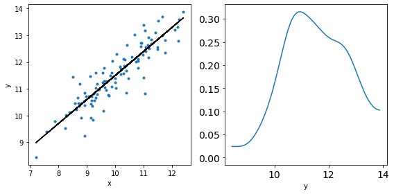
_, ax = plt.subplots(1,2,figsize=(8,4))
ax[0].plot(x,y,'C0.')
ax[0].set_xlabel('x')
ax[0].set_ylabel('y')
ax[0].plot(x,y_real,'k')
az.plot_kde(y,ax=ax[1])
ax[1].set_xlabel('y')
plt.tight_layout()

#!pip install pymc3

import pymc3 as pm

with pm.Model() as model_g:
    α = pm.Normal('α', mu=0, sd=10)
    β = pm.Normal('β', mu=0, sd=1)
    ϵ = pm.HalfCauchy('ϵ', 5)

    μ = pm.Deterministic('μ', α + β * x)
    y_pred = pm.Normal('y_pred', mu=α + β * x, sd=ϵ, observed=y)

    trace_g = pm.sample(2000, tune=1000, return_inferencedata=True)

Auto-assigning NUTS sampler...
Initializing NUTS using jitter+adapt_diag...
Multiprocess sampling (4 chains in 4 jobs)
NUTS: [ϵ, β, α]

100.00% [12000/12000 00:03<00:00 Sampling 4 chains, 0 divergences]

/Users/cfanelli/Desktop/teaching/BRDS/jupynb_env_new/lib/python3.9/site-packages/scipy/stats/_continuous_distns.py:624: RuntimeWarning: overflow encountered in _beta_ppf
  return _boost._beta_ppf(q, a, b)
/Users/cfanelli/Desktop/teaching/BRDS/jupynb_env_new/lib/python3.9/site-packages/scipy/stats/_continuous_distns.py:624: RuntimeWarning: overflow encountered in _beta_ppf
  return _boost._beta_ppf(q, a, b)
/Users/cfanelli/Desktop/teaching/BRDS/jupynb_env_new/lib/python3.9/site-packages/scipy/stats/_continuous_distns.py:624: RuntimeWarning: overflow encountered in _beta_ppf
  return _boost._beta_ppf(q, a, b)
/Users/cfanelli/Desktop/teaching/BRDS/jupynb_env_new/lib/python3.9/site-packages/scipy/stats/_continuous_distns.py:624: RuntimeWarning: overflow encountered in _beta_ppf
  return _boost._beta_ppf(q, a, b)
Sampling 4 chains for 1_000 tune and 2_000 draw iterations (4_000 + 8_000 draws total) took 9 seconds.

az.plot_trace(trace_g, var_names=['α', 'β', 'ϵ'])

array([[<AxesSubplot:title={'center':'α'}>,
        <AxesSubplot:title={'center':'α'}>],
       [<AxesSubplot:title={'center':'β'}>,
        <AxesSubplot:title={'center':'β'}>],
       [<AxesSubplot:title={'center':'ϵ'}>,
        <AxesSubplot:title={'center':'ϵ'}>]], dtype=object)

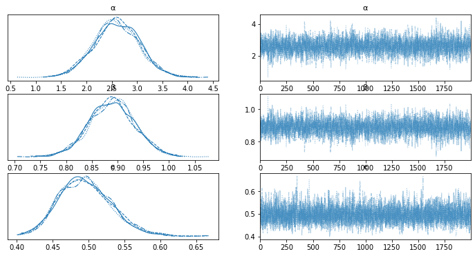
az.summary(trace_g)

	mean	sd	hdi_3%	hdi_97%	mcse_mean	mcse_sd	ess_bulk	ess_tail	r_hat
α	2.595	0.447	1.728	3.404	0.009	0.006	2733.0	3003.0	1.0
β	0.889	0.044	0.804	0.972	0.001	0.001	2707.0	3044.0	1.0
ϵ	0.496	0.036	0.431	0.566	0.001	0.000	3258.0	2847.0	1.0
μ[0]	10.524	0.070	10.398	10.662	0.001	0.001	3636.0	4872.0	1.0
μ[1]	12.377	0.065	12.252	12.498	0.001	0.001	4269.0	5502.0	1.0
...	...	...	...	...	...	...	...	...	...
μ[95]	12.407	0.066	12.280	12.530	0.001	0.001	4202.0	5346.0	1.0
μ[96]	10.525	0.070	10.399	10.663	0.001	0.001	3638.0	4872.0	1.0
μ[97]	10.277	0.079	10.130	10.426	0.001	0.001	3362.0	4434.0	1.0
μ[98]	11.828	0.052	11.729	11.925	0.001	0.000	6144.0	5820.0	1.0
μ[99]	11.153	0.053	11.053	11.250	0.001	0.001	5284.0	5478.0	1.0

103 rows × 9 columns

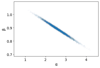
az.plot_pair(trace_g,var_names=['α','β'], scatter_kwargs={'alpha': 0.01})

<AxesSubplot:xlabel='α', ylabel='β'>

#plt.plot(x, y, 'C0.')

res = az.summary(trace_g)
alpha_m = res.loc['α']['mean']
beta_m  = res.loc['β']['mean']

#print(res)


trace_a = trace_g['posterior']['α'][0].values 
trace_b = trace_g['posterior']['β'][0].values 

draws = range(0, len(trace_g['posterior']['α'][0]), 10)


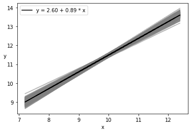
plt.plot(x, trace_a[draws] + trace_b[draws]
         * x[:, np.newaxis], c='gray', alpha=0.5);

plt.plot(x, alpha_m + beta_m * x, c='k',
         label=f'y = {alpha_m:.2f} + {beta_m:.2f} * x');

plt.xlabel('x')
plt.ylabel('y', rotation=0)
plt.legend();

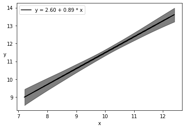
plt.plot(x, alpha_m + beta_m * x, c='k',
         label=f'y = {alpha_m:.2f} + {beta_m:.2f} * x')

sig = az.plot_hdi(x, trace_g.posterior['μ'], hdi_prob=0.999, color='k')

plt.xlabel('x')
plt.ylabel('y', rotation=0)
plt.legend()

<matplotlib.legend.Legend at 0x29ca0ffd0>

ppc = pm.sample_posterior_predictive(trace_g, samples=4000, model=model_g)

/Users/cfanelli/Desktop/teaching/BRDS/jupynb_env_new/lib/python3.9/site-packages/pymc3/sampling.py:1708: UserWarning: samples parameter is smaller than nchains times ndraws, some draws and/or chains may not be represented in the returned posterior predictive sample
  warnings.warn(

100.00% [4000/4000 00:01<00:00]

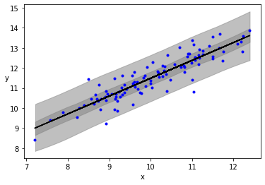
plt.plot(x, y, 'b.')


plt.plot(x, alpha_m + beta_m * x, c='k',
         label=f'y = {alpha_m:.2f} + {beta_m:.2f} * x')


az.plot_hdi(x, ppc['y_pred'], hdi_prob=0.5, color='gray')
az.plot_hdi(x, ppc['y_pred'], hdi_prob=0.98, color='gray')

plt.xlabel('x')
plt.ylabel('y', rotation=0)

/Users/cfanelli/Desktop/teaching/BRDS/jupynb_env_new/lib/python3.9/site-packages/arviz/plots/hdiplot.py:157: FutureWarning: hdi currently interprets 2d data as (draw, shape) but this will change in a future release to (chain, draw) for coherence with other functions
  hdi_data = hdi(y, hdi_prob=hdi_prob, circular=circular, multimodal=False, **hdi_kwargs)

Text(0, 0.5, 'y')

mus = res.loc[:]['mean'][3 :].values
hdi_3 = res.loc[:]['hdi_3%'][3 :].values
hdi_97 = res.loc[:]['hdi_97%'][3 :].values

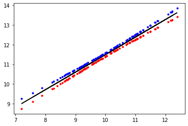
plt.plot(x, mus, c='k')
plt.plot(x,hdi_3, 'r.')
plt.plot(x,hdi_97, 'b.')
#plt.fill_between(x,hdi_3,hdi_97, facecolor = "red")

[<matplotlib.lines.Line2D at 0x29b7ab0a0>]

Comparison with Ordinary Least Sqaures

from scipy import stats

lreg = stats.linregress(x,y)

slope = lreg.slope
slope_err = lreg.stderr
interc = lreg.intercept
interc_err = lreg.intercept_stderr


res = az.summary(trace_g)
alpha_m = res.loc['α']['mean']
alpha_s = res.loc['α']['sd']
beta_m  = res.loc['β']['mean']
beta_s = res.loc['β']['sd']

print("\nOLS:\nα= {:1.3} +/- {:1.3}".format(interc,interc_err))
print("β= {:1.3} +/- {:1.3}\n".format(slope,slope_err))
print("\nBayesLR:\nα= {:1.3} +/- {:1.3}".format(alpha_m,alpha_s))
print("β= {:1.3} +/- {:1.3}\n".format(beta_m,beta_s))

OLS:
α= 2.57 +/- 0.438
β= 0.892 +/- 0.0434


BayesLR:
α= 2.6 +/- 0.447
β= 0.889 +/- 0.044

Exercise: Robust linear regression with Anscombe Dataset

import io
import csv 
import requests
import pandas as pd

target_url = 'https://raw.githubusercontent.com/cfteach/brds/main/datasets/anscombe.csv' 

download = requests.get(target_url).content
ans = pd.read_csv(io.StringIO(download.decode('utf-8')))


x_3 = ans[ans.group == 'III']['x'].values

x_3 = ans[ans.group == 'III']['x'].values
y_3 = ans[ans.group == 'III']['y'].values
x_3 = x_3 - x_3.mean()

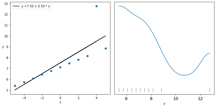
_, ax = plt.subplots(1, 2, figsize=(10, 5))
lreg = stats.linregress(x_3, y_3)

beta_c, alpha_c = lreg[:2]

ax[0].plot(x_3, (alpha_c + beta_c * x_3), 'k',
           label=f'y ={alpha_c:.2f} + {beta_c:.2f} * x')
ax[0].plot(x_3, y_3, 'C0o')
ax[0].set_xlabel('x')
ax[0].set_ylabel('y', rotation=0)
ax[0].legend(loc=0)
az.plot_kde(y_3, ax=ax[1], rug=True)
ax[1].set_xlabel('y')
ax[1].set_yticks([])
plt.tight_layout()

with pm.Model() as model_t:
    α = pm.Normal('α', mu=y_3.mean(), sd=1)
    β = pm.Normal('β', mu=0, sd=1)
    ϵ = pm.HalfNormal('ϵ', 5)
    ν_ = pm.Exponential('ν_', 1/29)
    ν = pm.Deterministic('ν', ν_ + 1) #a shifted exponential to avoid values of ν close to 0 

    y_pred = pm.StudentT('y_pred', mu=α + β * x_3,
                         sd=ϵ, nu=ν, observed=y_3)

    trace_t = pm.sample(5000, tune=1000, return_inferencedata=True)

Auto-assigning NUTS sampler...
Initializing NUTS using jitter+adapt_diag...
Multiprocess sampling (4 chains in 4 jobs)
NUTS: [ν_, ϵ, β, α]

100.00% [24000/24000 00:03<00:00 Sampling 4 chains, 0 divergences]

/Users/cfanelli/Desktop/teaching/BRDS/jupynb_env_new/lib/python3.9/site-packages/scipy/stats/_continuous_distns.py:624: RuntimeWarning: overflow encountered in _beta_ppf
  return _boost._beta_ppf(q, a, b)
/Users/cfanelli/Desktop/teaching/BRDS/jupynb_env_new/lib/python3.9/site-packages/scipy/stats/_continuous_distns.py:624: RuntimeWarning: overflow encountered in _beta_ppf
  return _boost._beta_ppf(q, a, b)
/Users/cfanelli/Desktop/teaching/BRDS/jupynb_env_new/lib/python3.9/site-packages/scipy/stats/_continuous_distns.py:624: RuntimeWarning: overflow encountered in _beta_ppf
  return _boost._beta_ppf(q, a, b)
/Users/cfanelli/Desktop/teaching/BRDS/jupynb_env_new/lib/python3.9/site-packages/scipy/stats/_continuous_distns.py:624: RuntimeWarning: overflow encountered in _beta_ppf
  return _boost._beta_ppf(q, a, b)
Sampling 4 chains for 1_000 tune and 5_000 draw iterations (4_000 + 20_000 draws total) took 8 seconds.
The number of effective samples is smaller than 25% for some parameters.

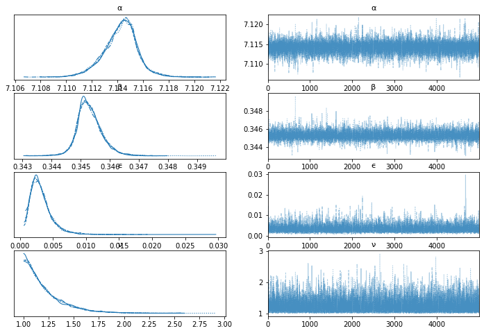
varnames = ['α', 'β', 'ϵ', 'ν']
az.plot_trace(trace_t, var_names=varnames);

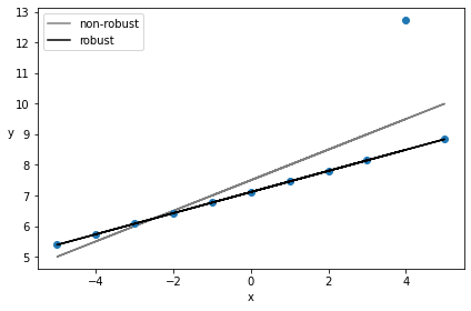
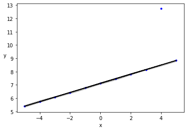
beta_c, alpha_c = stats.linregress(x_3, y_3)[:2]

rest = az.summary(trace_t)


plt.plot(x_3, (alpha_c + beta_c * x_3), 'k', label='non-robust', alpha=0.5)
plt.plot(x_3, y_3, 'C0o')
alpha_m = rest.loc['α']['mean']
beta_m  = rest.loc['β']['mean']
plt.plot(x_3, alpha_m + beta_m * x_3, c='k', label='robust')

plt.xlabel('x')
plt.ylabel('y', rotation=0)
plt.legend(loc=2)
plt.tight_layout()

az.summary(trace_t, var_names=varnames)

	mean	sd	hdi_3%	hdi_97%	mcse_mean	mcse_sd	ess_bulk	ess_tail	r_hat
α	7.114	0.001	7.112	7.117	0.000	0.000	10694.0	10221.0	1.0
β	0.345	0.000	0.345	0.346	0.000	0.000	9272.0	8380.0	1.0
ϵ	0.003	0.002	0.001	0.006	0.000	0.000	4064.0	2033.0	1.0
ν	1.212	0.203	1.000	1.581	0.002	0.001	7615.0	5699.0	1.0

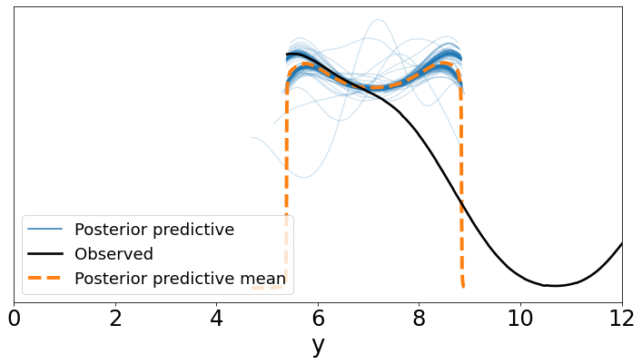
ppc = pm.sample_posterior_predictive(trace_t, samples=200, model=model_t, random_seed=2)

/Users/cfanelli/Desktop/teaching/BRDS/jupynb_env_new/lib/python3.9/site-packages/pymc3/sampling.py:1708: UserWarning: samples parameter is smaller than nchains times ndraws, some draws and/or chains may not be represented in the returned posterior predictive sample
  warnings.warn(

100.00% [200/200 00:00<00:00]

data_ppc = az.from_pymc3(posterior_predictive=ppc, model = model_t)
ax = az.plot_ppc(data_ppc, figsize=(12, 6), mean=True)
plt.xlim(0, 12)
plt.xlabel('y')

Text(0.5, 0, 'y')

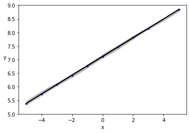
plt.plot(x_3, y_3, 'b.')

plt.plot(x_3, alpha_m + beta_m * x_3, c='k',
         label=f'y = {alpha_m:.2f} + {beta_m:.2f} * x')


az.plot_hdi(x_3, ppc['y_pred'], hdi_prob=0.5, color='gray')
az.plot_hdi(x_3, ppc['y_pred'], hdi_prob=0.98, color='gray')

plt.xlabel('x')
plt.ylabel('y', rotation=0)

/Users/cfanelli/Desktop/teaching/BRDS/jupynb_env_new/lib/python3.9/site-packages/arviz/plots/hdiplot.py:157: FutureWarning: hdi currently interprets 2d data as (draw, shape) but this will change in a future release to (chain, draw) for coherence with other functions
  hdi_data = hdi(y, hdi_prob=hdi_prob, circular=circular, multimodal=False, **hdi_kwargs)

Text(0, 0.5, 'y')

plt.ylim(5.,9.)

plt.plot(x_3, y_3, 'b.')

plt.plot(x_3, alpha_m + beta_m * x_3, c='k',
         label=f'y = {alpha_m:.2f} + {beta_m:.2f} * x')


az.plot_hdi(x_3, ppc['y_pred'], hdi_prob=0.5, color='gray')
az.plot_hdi(x_3, ppc['y_pred'], hdi_prob=0.98, color='gray')

plt.xlabel('x')
plt.ylabel('y', rotation=0)

Text(0, 0.5, 'y')