Logistic Regression

Ref: Chap 4 of Mar18

https://cfteach.github.io/brds/referencesmd.html

!pip install pymc3 

Looking in indexes: https://pypi.org/simple, https://us-python.pkg.dev/colab-wheels/public/simple/
Collecting pymc3
  Downloading pymc3-3.11.5-py3-none-any.whl (872 kB)
     |████████████████████████████████| 872 kB 12.8 MB/s 
?25hRequirement already satisfied: numpy<1.22.2,>=1.15.0 in /usr/local/lib/python3.7/dist-packages (from pymc3) (1.21.6)
Requirement already satisfied: dill in /usr/local/lib/python3.7/dist-packages (from pymc3) (0.3.6)
Collecting semver>=2.13.0
  Downloading semver-2.13.0-py2.py3-none-any.whl (12 kB)
Requirement already satisfied: arviz>=0.11.0 in /usr/local/lib/python3.7/dist-packages (from pymc3) (0.12.1)
Requirement already satisfied: cachetools>=4.2.1 in /usr/local/lib/python3.7/dist-packages (from pymc3) (5.2.0)
Requirement already satisfied: fastprogress>=0.2.0 in /usr/local/lib/python3.7/dist-packages (from pymc3) (1.0.3)
Collecting theano-pymc==1.1.2
  Downloading Theano-PyMC-1.1.2.tar.gz (1.8 MB)
     |████████████████████████████████| 1.8 MB 30.9 MB/s 
?25hRequirement already satisfied: typing-extensions>=3.7.4 in /usr/local/lib/python3.7/dist-packages (from pymc3) (4.1.1)
Collecting deprecat
  Downloading deprecat-2.1.1-py2.py3-none-any.whl (9.8 kB)
Requirement already satisfied: patsy>=0.5.1 in /usr/local/lib/python3.7/dist-packages (from pymc3) (0.5.3)
Requirement already satisfied: pandas>=0.24.0 in /usr/local/lib/python3.7/dist-packages (from pymc3) (1.3.5)
Requirement already satisfied: scipy<1.8.0,>=1.7.3 in /usr/local/lib/python3.7/dist-packages (from pymc3) (1.7.3)
Requirement already satisfied: filelock in /usr/local/lib/python3.7/dist-packages (from theano-pymc==1.1.2->pymc3) (3.8.0)
Requirement already satisfied: setuptools>=38.4 in /usr/local/lib/python3.7/dist-packages (from arviz>=0.11.0->pymc3) (57.4.0)
Requirement already satisfied: xarray>=0.16.1 in /usr/local/lib/python3.7/dist-packages (from arviz>=0.11.0->pymc3) (0.20.2)
Requirement already satisfied: xarray-einstats>=0.2 in /usr/local/lib/python3.7/dist-packages (from arviz>=0.11.0->pymc3) (0.2.2)
Requirement already satisfied: matplotlib>=3.0 in /usr/local/lib/python3.7/dist-packages (from arviz>=0.11.0->pymc3) (3.2.2)
Requirement already satisfied: netcdf4 in /usr/local/lib/python3.7/dist-packages (from arviz>=0.11.0->pymc3) (1.6.1)
Requirement already satisfied: packaging in /usr/local/lib/python3.7/dist-packages (from arviz>=0.11.0->pymc3) (21.3)
Requirement already satisfied: kiwisolver>=1.0.1 in /usr/local/lib/python3.7/dist-packages (from matplotlib>=3.0->arviz>=0.11.0->pymc3) (1.4.4)
Requirement already satisfied: pyparsing!=2.0.4,!=2.1.2,!=2.1.6,>=2.0.1 in /usr/local/lib/python3.7/dist-packages (from matplotlib>=3.0->arviz>=0.11.0->pymc3) (3.0.9)
Requirement already satisfied: python-dateutil>=2.1 in /usr/local/lib/python3.7/dist-packages (from matplotlib>=3.0->arviz>=0.11.0->pymc3) (2.8.2)
Requirement already satisfied: cycler>=0.10 in /usr/local/lib/python3.7/dist-packages (from matplotlib>=3.0->arviz>=0.11.0->pymc3) (0.11.0)
Requirement already satisfied: pytz>=2017.3 in /usr/local/lib/python3.7/dist-packages (from pandas>=0.24.0->pymc3) (2022.6)
Requirement already satisfied: six in /usr/local/lib/python3.7/dist-packages (from patsy>=0.5.1->pymc3) (1.15.0)
Requirement already satisfied: importlib-metadata in /usr/local/lib/python3.7/dist-packages (from xarray>=0.16.1->arviz>=0.11.0->pymc3) (4.13.0)
Requirement already satisfied: wrapt<2,>=1.10 in /usr/local/lib/python3.7/dist-packages (from deprecat->pymc3) (1.14.1)
Requirement already satisfied: zipp>=0.5 in /usr/local/lib/python3.7/dist-packages (from importlib-metadata->xarray>=0.16.1->arviz>=0.11.0->pymc3) (3.10.0)
Requirement already satisfied: cftime in /usr/local/lib/python3.7/dist-packages (from netcdf4->arviz>=0.11.0->pymc3) (1.6.2)
Building wheels for collected packages: theano-pymc
  Building wheel for theano-pymc (setup.py) ... ?25l?25hdone
  Created wheel for theano-pymc: filename=Theano_PyMC-1.1.2-py3-none-any.whl size=1529964 sha256=defebffb659cb5ed16c8f722ef3988e92655cced11359b7b4bebf871f2b9ba9f
  Stored in directory: /root/.cache/pip/wheels/f3/af/8c/5dd7553522d74c52a7813806fc7ee1a9caa20a3f7c8fd850d5
Successfully built theano-pymc
Installing collected packages: theano-pymc, semver, deprecat, pymc3
Successfully installed deprecat-2.1.1 pymc3-3.11.5 semver-2.13.0 theano-pymc-1.1.2

import pymc3 as pm
import numpy as np
import pandas as pd
import theano.tensor as tt
import seaborn as sns
import scipy.stats as stats
from scipy.special import expit as logistic
import matplotlib.pyplot as plt
import arviz as az
import requests
import io 

az.style.use('arviz-darkgrid')

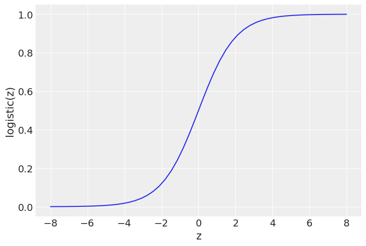
z = np.linspace(-8, 8)
plt.plot(z, 1 / (1 + np.exp(-z)))
plt.xlabel('z')
plt.ylabel('logistic(z)')

Text(0, 0.5, 'logistic(z)')

The Iris Dataset

target_url = 'https://raw.githubusercontent.com/cfteach/brds/main/datasets/iris.csv' 

download = requests.get(target_url).content
iris = pd.read_csv(io.StringIO(download.decode('utf-8')))

iris.head()

	sepal_length	sepal_width	petal_length	petal_width	species
0	5.1	3.5	1.4	0.2	setosa
1	4.9	3.0	1.4	0.2	setosa
2	4.7	3.2	1.3	0.2	setosa
3	4.6	3.1	1.5	0.2	setosa
4	5.0	3.6	1.4	0.2	setosa

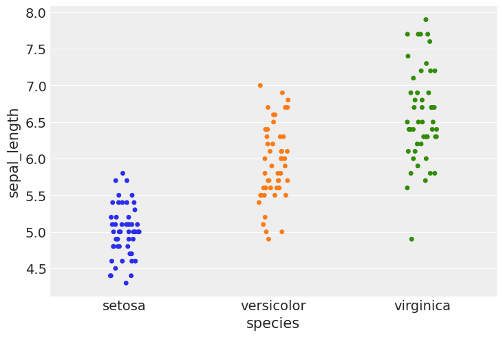
#using stripplot function from seaborn 

sns.stripplot(x="species", y="sepal_length", data=iris, jitter=True)

<matplotlib.axes._subplots.AxesSubplot at 0x7f5290a34350>

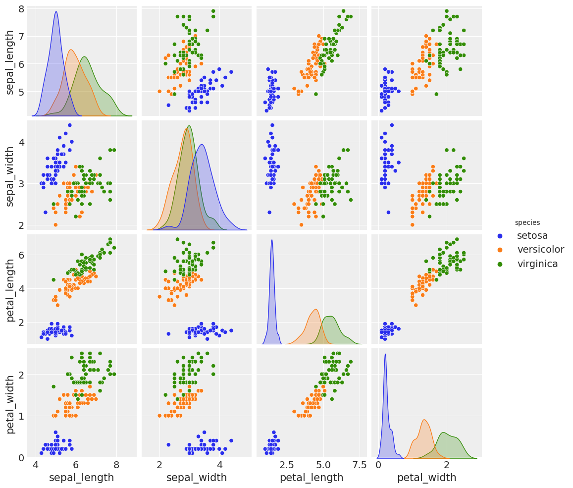
sns.pairplot(iris, hue='species', diag_kind='kde')

/usr/local/lib/python3.7/dist-packages/seaborn/axisgrid.py:88: UserWarning: This figure was using constrained_layout==True, but that is incompatible with subplots_adjust and or tight_layout: setting constrained_layout==False. 
  self._figure.tight_layout(*args, **kwargs)

<seaborn.axisgrid.PairGrid at 0x7f52909aeb10>

The logistic model applied to the iris dataset

df = iris.query("species == ('setosa', 'versicolor')")

df

	sepal_length	sepal_width	petal_length	petal_width	species
0	5.1	3.5	1.4	0.2	setosa
1	4.9	3.0	1.4	0.2	setosa
2	4.7	3.2	1.3	0.2	setosa
3	4.6	3.1	1.5	0.2	setosa
4	5.0	3.6	1.4	0.2	setosa
...	...	...	...	...	...
95	5.7	3.0	4.2	1.2	versicolor
96	5.7	2.9	4.2	1.3	versicolor
97	6.2	2.9	4.3	1.3	versicolor
98	5.1	2.5	3.0	1.1	versicolor
99	5.7	2.8	4.1	1.3	versicolor

100 rows × 5 columns

y_0 = pd.Categorical(df['species']).codes

print(y_0, len(y_0))

[0 0 0 0 0 0 0 0 0 0 0 0 0 0 0 0 0 0 0 0 0 0 0 0 0 0 0 0 0 0 0 0 0 0 0 0 0
 0 0 0 0 0 0 0 0 0 0 0 0 0 1 1 1 1 1 1 1 1 1 1 1 1 1 1 1 1 1 1 1 1 1 1 1 1
 1 1 1 1 1 1 1 1 1 1 1 1 1 1 1 1 1 1 1 1 1 1 1 1 1 1] 100

# let's select one variate
x_n = 'sepal_length'
x_0 = df[x_n].values
#print(x_0)

# let's center our dataset, as we have done in other exercises
x_c = x_0 - x_0.mean()
print(x_c)

[-0.371 -0.571 -0.771 -0.871 -0.471 -0.071 -0.871 -0.471 -1.071 -0.571
 -0.071 -0.671 -0.671 -1.171  0.329  0.229 -0.071 -0.371  0.229 -0.371
 -0.071 -0.371 -0.871 -0.371 -0.671 -0.471 -0.471 -0.271 -0.271 -0.771
 -0.671 -0.071 -0.271  0.029 -0.571 -0.471  0.029 -0.571 -1.071 -0.371
 -0.471 -0.971 -1.071 -0.471 -0.371 -0.671 -0.371 -0.871 -0.171 -0.471
  1.529  0.929  1.429  0.029  1.029  0.229  0.829 -0.571  1.129 -0.271
 -0.471  0.429  0.529  0.629  0.129  1.229  0.129  0.329  0.729  0.129
  0.429  0.629  0.829  0.629  0.929  1.129  1.329  1.229  0.529  0.229
  0.029  0.029  0.329  0.529 -0.071  0.529  1.229  0.829  0.129  0.029
  0.029  0.629  0.329 -0.471  0.129  0.229  0.229  0.729 -0.371  0.229]

with pm.Model() as model_0:
    α = pm.Normal('α', mu=0, sd=10)
    β = pm.Normal('β', mu=0, sd=10)
    
    μ = α + pm.math.dot(x_c, β)    
    θ = pm.Deterministic('θ', pm.math.sigmoid(μ))
    bd = pm.Deterministic('bd', -α/β)
    
    yl = pm.Bernoulli('yl', p=θ, observed=y_0)

    trace_0 = pm.sample(2000, tune = 2000, return_inferencedata=True)

100.00% [4000/4000 00:05<00:00 Sampling chain 0, 0 divergences]

100.00% [4000/4000 00:02<00:00 Sampling chain 1, 0 divergences]

varnames = ['α', 'β', 'bd']
res = az.summary(trace_0)
#print(res)
az.summary(trace_0)

	mean	sd	hdi_3%	hdi_97%	mcse_mean	mcse_sd	ess_bulk	ess_tail	r_hat
α	0.309	0.351	-0.345	0.955	0.006	0.005	2972.0	2475.0	1.0
β	5.409	1.047	3.469	7.348	0.021	0.015	2655.0	2333.0	1.0
θ[0]	0.164	0.060	0.060	0.277	0.001	0.001	3071.0	2506.0	1.0
θ[1]	0.068	0.037	0.011	0.135	0.001	0.000	2948.0	2406.0	1.0
θ[2]	0.027	0.021	0.001	0.064	0.000	0.000	2867.0	2277.0	1.0
...	...	...	...	...	...	...	...	...	...
θ[96]	0.815	0.067	0.689	0.930	0.001	0.001	2727.0	2186.0	1.0
θ[97]	0.980	0.018	0.947	0.999	0.000	0.000	2609.0	2140.0	1.0
θ[98]	0.164	0.060	0.060	0.277	0.001	0.001	3071.0	2506.0	1.0
θ[99]	0.815	0.067	0.689	0.930	0.001	0.001	2727.0	2186.0	1.0
bd	-0.056	0.065	-0.170	0.070	0.001	0.001	3016.0	2591.0	1.0

103 rows × 9 columns

theta_post= trace_0.posterior['θ'] 
print(np.shape(theta_post))

(2, 2000, 100)

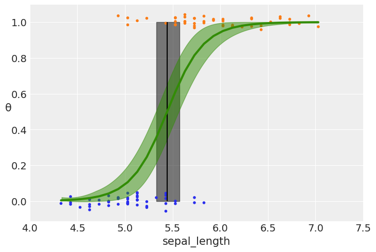
theta = trace_0.posterior['θ'].mean(axis=0).mean(axis=0)
idx = np.argsort(x_c)

np.random.seed(123)


plt.plot(x_c[idx], theta[idx], color='C2', lw=3)

plt.vlines(trace_0.posterior['bd'].mean(), 0, 1, color='k')

bd_hpd = az.hdi(trace_0.posterior['bd'])


plt.fill_betweenx([0, 1], bd_hpd.bd[0].values, bd_hpd.bd[1].values, color='k', alpha=0.5)


plt.scatter(x_c, np.random.normal(y_0, 0.02),
            marker='.', color=[f'C{x}' for x in y_0])


az.plot_hdi(x_c, trace_0.posterior['θ'], color='C2')  #green band 


plt.xlabel(x_n)
plt.ylabel('θ', rotation=0)
# use original scale for xticks
locs, _ = plt.xticks()
plt.xticks(locs, np.round(locs + x_0.mean(), 1))

([<matplotlib.axis.XTick at 0x7f5280db0250>,
  <matplotlib.axis.XTick at 0x7f5280db0090>,
  <matplotlib.axis.XTick at 0x7f5280e10fd0>,
  <matplotlib.axis.XTick at 0x7f5280d0c5d0>,
  <matplotlib.axis.XTick at 0x7f5280d0cdd0>,
  <matplotlib.axis.XTick at 0x7f5280d0cd50>,
  <matplotlib.axis.XTick at 0x7f5280d0c590>,
  <matplotlib.axis.XTick at 0x7f5280d11810>],
 [Text(0, 0, '4.0'),
  Text(0, 0, '4.5'),
  Text(0, 0, '5.0'),
  Text(0, 0, '5.5'),
  Text(0, 0, '6.0'),
  Text(0, 0, '6.5'),
  Text(0, 0, '7.0'),
  Text(0, 0, '7.5')])

Multiple logistic regression

df = iris.query("species == ('setosa', 'versicolor')") 
y_1 = pd.Categorical(df['species']).codes 
x_n = ['sepal_length', 'sepal_width'] 
x_1 = df[x_n].values

print(np.shape(x_1), type(x_1))
t_l = x_1.tolist()
print(np.shape(t_l), type(t_l))

(100, 2) <class 'numpy.ndarray'>
(100, 2) <class 'list'>

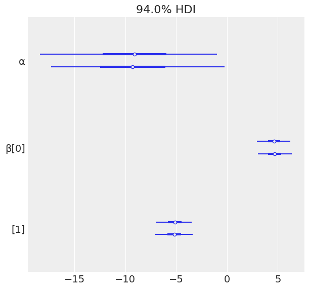
with pm.Model() as model_1: 
    α = pm.Normal('α', mu=0, sd=10) 
    β = pm.Normal('β', mu=0, sd=2, shape=len(x_n)) 

    x__1 = pm.Data('x', x_1)
    y__1 = pm.Data('y', y_1)
     
    μ = α + pm.math.dot(x__1, β)
    
    θ = pm.Deterministic('θ', 1 / (1 + pm.math.exp(-μ))) 
    bd = pm.Deterministic('bd', -α/β[1] - β[0]/β[1] * x__1[:,0])
     
    yl = pm.Bernoulli('yl', p=θ, observed=y__1) 
 
    trace_1 = pm.sample(2000, tune=4000, return_inferencedata=True, target_accept=0.9)

100.00% [6000/6000 00:29<00:00 Sampling chain 0, 0 divergences]

100.00% [6000/6000 00:29<00:00 Sampling chain 1, 0 divergences]

varnames = ['α', 'β'] 
az.plot_forest(trace_1, var_names=varnames);

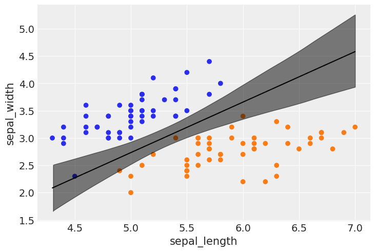
idx = np.argsort(x_1[:,0]) 


bd_mean = trace_1.posterior['bd'].mean(axis=0).mean(axis=0)


plt.scatter(x_1[:,0], x_1[:,1], c=[f'C{x}' for x in y_0]) 

bd = bd_mean[idx]

plt.plot(x_1[:,0][idx], bd, color='k'); 


az.plot_hdi(x_1[:,0], trace_1.posterior['bd'], color='k')
 
    
plt.xlabel(x_n[0]) 
plt.ylabel(x_n[1])

Text(0, 0.5, 'sepal_width')

Prediction on unseen data

print(np.shape(x_1), type(x_1))

udata = np.array(((5.2,2.0),(7.0,2.0),(4.5,5.0),(5.5,3.2)))

print(np.shape(udata), type(udata))


#dic = {'x_1': udata[:,0].tolist(), 'sepal_width': udata[:,1].tolist()}
tmp_dic = {'x': udata}
#a=udata[:,0].tolist()
#print(type(a))
#print(a)

(100, 2) <class 'numpy.ndarray'>
(4, 2) <class 'numpy.ndarray'>

with model_1:
  pm.set_data(tmp_dic)
  y_test = pm.sample_posterior_predictive(trace_1, 200, model_1)

/usr/local/lib/python3.7/dist-packages/pymc3/sampling.py:1709: UserWarning: samples parameter is smaller than nchains times ndraws, some draws and/or chains may not be represented in the returned posterior predictive sample
  "samples parameter is smaller than nchains times ndraws, some draws "

100.00% [200/200 00:04<00:00]

print(np.shape(y_test['yl']), type(y_test['yl']))
res = y_test['yl'].mean(axis=0)
#res = np.round(y_test['yl'].mean(axis=0), decimals=0).astype(int)


for i,k in enumerate(udata):
  print('sepal_length, sepal_width, category: {:}, {:}'.format(udata[i], res[i]))

(200, 4) <class 'numpy.ndarray'>
sepal_length, sepal_width, category: [5.2 2. ], 0.99
sepal_length, sepal_width, category: [7. 2.], 1.0
sepal_length, sepal_width, category: [4.5 5. ], 0.0
sepal_length, sepal_width, category: [5.5 3.2], 0.425

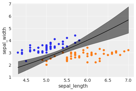
Question in class (from D. Zhu): why is the decision boundary linear?

with pm.Model() as model_2: 
    α = pm.Normal('α', mu=0, sd=10) 
    β = pm.Normal('β', mu=0, sd=2, shape=len(x_n)) 
    𝛾 = pm.Normal('𝛾', mu=0, sd=2) 
     
    μ = α + pm.math.dot(x_1, β) + pm.math.dot(x_1[:,0]**2, 𝛾)
    
    θ = pm.Deterministic('θ', 1 / (1 + pm.math.exp(-μ))) 
    bd = pm.Deterministic('bd', -α/β[1] - β[0]/β[1] * x_1[:,0] - 𝛾/β[1] * x_1[:,0]**2)
     
    yl = pm.Bernoulli('yl', p=θ, observed=y_1) 
 
    trace_2 = pm.sample(2000, tune=4000, return_inferencedata=True, target_accept=0.95)

Auto-assigning NUTS sampler...
Initializing NUTS using jitter+adapt_diag...
Multiprocess sampling (4 chains in 4 jobs)
NUTS: [𝛾, β, α]

100.00% [24000/24000 00:19<00:00 Sampling 4 chains, 0 divergences]

/Users/cfanelli/Desktop/teaching/BRDS/jupynb_env_new/lib/python3.9/site-packages/scipy/stats/_continuous_distns.py:624: RuntimeWarning: overflow encountered in _beta_ppf
  return _boost._beta_ppf(q, a, b)
/Users/cfanelli/Desktop/teaching/BRDS/jupynb_env_new/lib/python3.9/site-packages/scipy/stats/_continuous_distns.py:624: RuntimeWarning: overflow encountered in _beta_ppf
  return _boost._beta_ppf(q, a, b)
/Users/cfanelli/Desktop/teaching/BRDS/jupynb_env_new/lib/python3.9/site-packages/scipy/stats/_continuous_distns.py:624: RuntimeWarning: overflow encountered in _beta_ppf
  return _boost._beta_ppf(q, a, b)
/Users/cfanelli/Desktop/teaching/BRDS/jupynb_env_new/lib/python3.9/site-packages/scipy/stats/_continuous_distns.py:624: RuntimeWarning: overflow encountered in _beta_ppf
  return _boost._beta_ppf(q, a, b)
Sampling 4 chains for 4_000 tune and 2_000 draw iterations (16_000 + 8_000 draws total) took 26 seconds.

idx = np.argsort(x_1[:,0]) 


bd_mean = trace_2.posterior['bd'].mean(axis=0).mean(axis=0)


plt.scatter(x_1[:,0], x_1[:,1], c=[f'C{x}' for x in y_0]) 

bd = bd_mean[idx]

plt.plot(x_1[:,0][idx], bd, color='k'); 


az.plot_hdi(x_1[:,0], trace_2.posterior['bd'], color='k')
 
    
plt.xlabel(x_n[0]) 
plt.ylabel(x_n[1])

Text(0, 0.5, 'sepal_width')

y_pred_2 = pm.sample_posterior_predictive(trace_2, 200, model_2) 

/Users/cfanelli/Desktop/teaching/BRDS/jupynb_env_new/lib/python3.9/site-packages/pymc3/sampling.py:1708: UserWarning: samples parameter is smaller than nchains times ndraws, some draws and/or chains may not be represented in the returned posterior predictive sample
  warnings.warn(

100.00% [200/200 00:00<00:00]

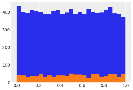
How to plot a variate distributed according to a PyMC model

with pm.Model() as model_testv:
    testv = pm.Beta('testv',1.,1.)
    


syn1 = testv.random(size=10000)
plt.hist(syn1, bins=25);

syn2 = testv.random(size=1000)
plt.hist(syn2, bins=25);