Metrics of Performance
Contents
Metrics of Performance#
The performance of a given tracker is characterized by more than 1 metric. For instance, EIC detector 1 tracker setup was evaluated against the following objectives.
Momentum resolution \(\sigma (\frac{\Delta p}{p})\)
Tip
Details about fitting and stability of the fits are discussed in detail in [2]
Angular resolution \(\sigma (\Delta \theta)\) & \(\sigma (\Delta \phi)\)
Angular resolution at PID detector locations \(\sigma (d\theta)\) & \(\sigma (d\phi)\)
\(DCA_{2D}\) resolution \(\sigma (d DCA_{2D})\)
Metric to evaluate vertex reconstruction.
Kalman Filter InEfficiency
Metric to evaluate the ability to reconstruct tracks
(4)#\[ R(\textup{KF}) = \frac{\textup{N(tracks not reconstructed)}}{\textup{N(total number of tracks)}}\]
Note
Not all the objectives above are simultaneously optimized in a single optimization. Combinations of above mentioned objectives are optimized simultaneously over various optimization pipelines. Many iterations are run in seperate pipelines as mentioned in Optimization as a continuous process
Calculating objectives#
Since the objectives depend on the kinematics and are calculated in 5 main bins in pseudorapidity (\(\eta\)): (i) \(-3.5 \leq \eta < -2.0\) (corresponding to the electron-going direction), (ii) -\(2.0 \leq \eta < -1.0\) (the transition region in electron-going direction), (iii) \(-1 \leq \eta < 1\) (the central barrel), (iv) \(1 \leq \eta < 2.0\) (the transition region in the hadron-going direction) and (v) \(2.0 \leq \eta < 3.5\) (the hadron-going direction). The rationale behind this binning is a combination of different aspects: the correspondence with the binning in the EIC Yellow Report [1], the asymmetric arrangement of detectors in electron-going and hadron-going directions and the division in pseudorapidity between the barrel region and the endcap. Particular attention is given to the transition region be- tween barrel and endcaps as well as at large \(|\eta| ∼ 3.5\) close to the beamline.
Charged pions are generated uniformly in the phase-space that covers the range in momentum magnitude \(p\) \(\in\) [0,20] GeV/c and the range in pseudorapidity \(\eta\) \(\in\) (-3.5,3.5)
Particular attention is given to the transition region between barrel and endcaps as well as at large \(|\eta| \sim\) 3.5 close to the beamline.
We generate statistics ranging from \(120k\) events to \(250k\) events which contains 5 \(pi^{-}\) tracks in each event.
To compute the objective metric, we need to combine the results from all the \(p\) and \(\eta\) bins. Also, Note that the optimization aims in finding design solutions that are performing better than the reference design, Therefore, the following expression (5) is defined as the objective metric, which comprises of ratio of objectives in each of the \(p\) and \(\eta\) bin between the current evaluated design point to its reference. Figure Fig. 5 shows visually how the objective metric is computed.
Note
Kalman Filter Inefficiency is not calculated as ratios but is calculated in its absolute value. This was empirically found to be more efficient.
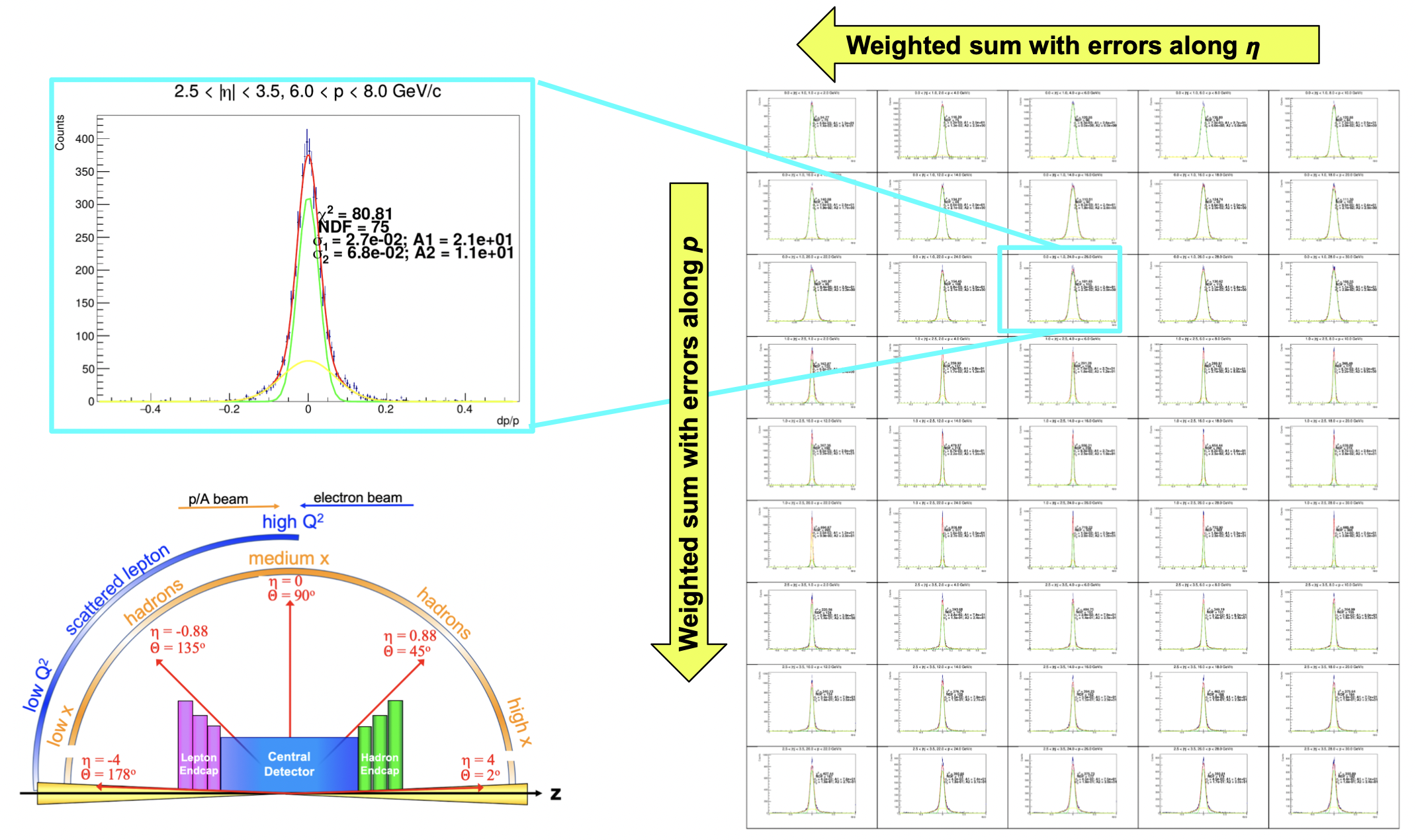
Fig. 5 Calculating Objective metric from various bins of \(\eta\) and \(p\). From the resolutions extracted from reference and the current design solution, ratios are formed and objective metric is calculated.#
Constraints#
Design parameters of the detector often are constrained due to various engineering reasons. For instance, the FST disks is made of ITS3- Silicon tiles stitched together, Therefore, the radius of the disks are constrained (Rmax - Rmin). Similarly, the minimum distance between the disks has to alteast 10cm to incorporate services.
One can encode these constraints into an Multi Objective Optimization problem ( Lecture 2 ). This ensures that during the process of optimization the algorithm will exclude the design space which are infeasible and generate solutions that minimally violate constraints.
For the tracker problem however, we introduce 2 types of contraints, Strong and soft constraints.
Strong Constraints#
These are constraints that cannot be violated at all. For instance, the minimum distance between 2 disks has to be atleast 10cm is a engineering requirement and always has to be respected. Therefore, these constraints heavily penalize the solutions and make sure, no optimizer will generator no design point violating this condition.
sub-detector |
constraint |
description |
|---|---|---|
EST/FST disks |
\(z_{n+1} - z_{n} >= 10.0\) cm |
minimum distance between 2 consecutive disks |
\(\mu\)RWELL |
\(r_{n+1} - r_{n} >= 5.0\) cm |
minimum distance between \(\mu\)Rwell barrel layers |
Soft constraints#
These are constraints that are allowed to minimally be violated. For instance the same case of the tiling of the FST disks, the radius we know are constrained however, the constraint on the radius depends on how the tiles are being arranged on the disk. Therefore, while we want to respect the constraint most of the time, we could allow minimal violation of constraints in order to increase our search space.
sub-detector |
constraint |
description |
|---|---|---|
EST/FST disks |
\(min \Bigg\{ \sum_{i}^{disks} \Bigg| \frac{R^{i}_{out} - R^{i}_{in}}{d} - \floor*{\frac{R^{i}_{out} - R^{i}_{in}}{d}} \Bigg| \Bigg\}\) |
sum of residuals in sensor coverage for disks; sensor dimensions: \(d\) = 17.8 (30.0) mm |
sagitta layers |
\( min\Bigg\{ \Bigg| \frac{2 \pi r_{sagitta}}{w} - \floor*{\frac{2 \pi r_{sagitta}}{w}} \Bigg| \Bigg\}\) |
residual in sensor coverage for every layer; sensor strip width: \(w\) = 17.8 mm |
- 1
et.al Khalek, R. Science requirements and detector concepts for the electron-ion collider: eic yellow report. 2021. URL: https://arxiv.org/abs/2103.05419, doi:10.48550/ARXIV.2103.05419.
- 2
C. Fanelli, Z. Papandreou, and et. al Suresh. Ai-assisted optimization of the ecce tracking system at the electron ion collider. 2022. URL: https://arxiv.org/abs/2205.09185, doi:10.48550/ARXIV.2205.09185.
- 3
J. Blank and K. Deb. Pymoo: multi-objective optimization in python. IEEE Access, 8():89497–89509, 2020.