Implementing a GNN using the PyTorch Geometric library

28. Implementing a GNN using the PyTorch Geometric library#

!pip install torch torchvision torchaudio torch-geometric networkx matplotlib

Requirement already satisfied: torch in /usr/local/lib/python3.11/dist-packages (2.6.0+cu124)
Requirement already satisfied: torchvision in /usr/local/lib/python3.11/dist-packages (0.21.0+cu124)
Requirement already satisfied: torchaudio in /usr/local/lib/python3.11/dist-packages (2.6.0+cu124)
Collecting torch-geometric
  Downloading torch_geometric-2.6.1-py3-none-any.whl.metadata (63 kB)
     ━━━━━━━━━━━━━━━━━━━━━━━━━━━━━━━━━━━━━━━━ 63.1/63.1 kB 3.3 MB/s eta 0:00:00
?25hRequirement already satisfied: networkx in /usr/local/lib/python3.11/dist-packages (3.4.2)
Requirement already satisfied: matplotlib in /usr/local/lib/python3.11/dist-packages (3.10.0)
Requirement already satisfied: filelock in /usr/local/lib/python3.11/dist-packages (from torch) (3.18.0)
Requirement already satisfied: typing-extensions>=4.10.0 in /usr/local/lib/python3.11/dist-packages (from torch) (4.13.2)
Requirement already satisfied: jinja2 in /usr/local/lib/python3.11/dist-packages (from torch) (3.1.6)
Requirement already satisfied: fsspec in /usr/local/lib/python3.11/dist-packages (from torch) (2025.3.2)
Collecting nvidia-cuda-nvrtc-cu12==12.4.127 (from torch)
  Downloading nvidia_cuda_nvrtc_cu12-12.4.127-py3-none-manylinux2014_x86_64.whl.metadata (1.5 kB)
Collecting nvidia-cuda-runtime-cu12==12.4.127 (from torch)
  Downloading nvidia_cuda_runtime_cu12-12.4.127-py3-none-manylinux2014_x86_64.whl.metadata (1.5 kB)
Collecting nvidia-cuda-cupti-cu12==12.4.127 (from torch)
  Downloading nvidia_cuda_cupti_cu12-12.4.127-py3-none-manylinux2014_x86_64.whl.metadata (1.6 kB)
Collecting nvidia-cudnn-cu12==9.1.0.70 (from torch)
  Downloading nvidia_cudnn_cu12-9.1.0.70-py3-none-manylinux2014_x86_64.whl.metadata (1.6 kB)
Collecting nvidia-cublas-cu12==12.4.5.8 (from torch)
  Downloading nvidia_cublas_cu12-12.4.5.8-py3-none-manylinux2014_x86_64.whl.metadata (1.5 kB)
Collecting nvidia-cufft-cu12==11.2.1.3 (from torch)
  Downloading nvidia_cufft_cu12-11.2.1.3-py3-none-manylinux2014_x86_64.whl.metadata (1.5 kB)
Collecting nvidia-curand-cu12==10.3.5.147 (from torch)
  Downloading nvidia_curand_cu12-10.3.5.147-py3-none-manylinux2014_x86_64.whl.metadata (1.5 kB)
Collecting nvidia-cusolver-cu12==11.6.1.9 (from torch)
  Downloading nvidia_cusolver_cu12-11.6.1.9-py3-none-manylinux2014_x86_64.whl.metadata (1.6 kB)
Collecting nvidia-cusparse-cu12==12.3.1.170 (from torch)
  Downloading nvidia_cusparse_cu12-12.3.1.170-py3-none-manylinux2014_x86_64.whl.metadata (1.6 kB)
Requirement already satisfied: nvidia-cusparselt-cu12==0.6.2 in /usr/local/lib/python3.11/dist-packages (from torch) (0.6.2)
Requirement already satisfied: nvidia-nccl-cu12==2.21.5 in /usr/local/lib/python3.11/dist-packages (from torch) (2.21.5)
Requirement already satisfied: nvidia-nvtx-cu12==12.4.127 in /usr/local/lib/python3.11/dist-packages (from torch) (12.4.127)
Collecting nvidia-nvjitlink-cu12==12.4.127 (from torch)
  Downloading nvidia_nvjitlink_cu12-12.4.127-py3-none-manylinux2014_x86_64.whl.metadata (1.5 kB)
Requirement already satisfied: triton==3.2.0 in /usr/local/lib/python3.11/dist-packages (from torch) (3.2.0)
Requirement already satisfied: sympy==1.13.1 in /usr/local/lib/python3.11/dist-packages (from torch) (1.13.1)
Requirement already satisfied: mpmath<1.4,>=1.1.0 in /usr/local/lib/python3.11/dist-packages (from sympy==1.13.1->torch) (1.3.0)
Requirement already satisfied: numpy in /usr/local/lib/python3.11/dist-packages (from torchvision) (2.0.2)
Requirement already satisfied: pillow!=8.3.*,>=5.3.0 in /usr/local/lib/python3.11/dist-packages (from torchvision) (11.1.0)
Requirement already satisfied: aiohttp in /usr/local/lib/python3.11/dist-packages (from torch-geometric) (3.11.15)
Requirement already satisfied: psutil>=5.8.0 in /usr/local/lib/python3.11/dist-packages (from torch-geometric) (5.9.5)
Requirement already satisfied: pyparsing in /usr/local/lib/python3.11/dist-packages (from torch-geometric) (3.2.3)
Requirement already satisfied: requests in /usr/local/lib/python3.11/dist-packages (from torch-geometric) (2.32.3)
Requirement already satisfied: tqdm in /usr/local/lib/python3.11/dist-packages (from torch-geometric) (4.67.1)
Requirement already satisfied: contourpy>=1.0.1 in /usr/local/lib/python3.11/dist-packages (from matplotlib) (1.3.2)
Requirement already satisfied: cycler>=0.10 in /usr/local/lib/python3.11/dist-packages (from matplotlib) (0.12.1)
Requirement already satisfied: fonttools>=4.22.0 in /usr/local/lib/python3.11/dist-packages (from matplotlib) (4.57.0)
Requirement already satisfied: kiwisolver>=1.3.1 in /usr/local/lib/python3.11/dist-packages (from matplotlib) (1.4.8)
Requirement already satisfied: packaging>=20.0 in /usr/local/lib/python3.11/dist-packages (from matplotlib) (24.2)
Requirement already satisfied: python-dateutil>=2.7 in /usr/local/lib/python3.11/dist-packages (from matplotlib) (2.8.2)
Requirement already satisfied: six>=1.5 in /usr/local/lib/python3.11/dist-packages (from python-dateutil>=2.7->matplotlib) (1.17.0)
Requirement already satisfied: aiohappyeyeballs>=2.3.0 in /usr/local/lib/python3.11/dist-packages (from aiohttp->torch-geometric) (2.6.1)
Requirement already satisfied: aiosignal>=1.1.2 in /usr/local/lib/python3.11/dist-packages (from aiohttp->torch-geometric) (1.3.2)
Requirement already satisfied: attrs>=17.3.0 in /usr/local/lib/python3.11/dist-packages (from aiohttp->torch-geometric) (25.3.0)
Requirement already satisfied: frozenlist>=1.1.1 in /usr/local/lib/python3.11/dist-packages (from aiohttp->torch-geometric) (1.5.0)
Requirement already satisfied: multidict<7.0,>=4.5 in /usr/local/lib/python3.11/dist-packages (from aiohttp->torch-geometric) (6.4.3)
Requirement already satisfied: propcache>=0.2.0 in /usr/local/lib/python3.11/dist-packages (from aiohttp->torch-geometric) (0.3.1)
Requirement already satisfied: yarl<2.0,>=1.17.0 in /usr/local/lib/python3.11/dist-packages (from aiohttp->torch-geometric) (1.19.0)
Requirement already satisfied: MarkupSafe>=2.0 in /usr/local/lib/python3.11/dist-packages (from jinja2->torch) (3.0.2)
Requirement already satisfied: charset-normalizer<4,>=2 in /usr/local/lib/python3.11/dist-packages (from requests->torch-geometric) (3.4.1)
Requirement already satisfied: idna<4,>=2.5 in /usr/local/lib/python3.11/dist-packages (from requests->torch-geometric) (3.10)
Requirement already satisfied: urllib3<3,>=1.21.1 in /usr/local/lib/python3.11/dist-packages (from requests->torch-geometric) (2.3.0)
Requirement already satisfied: certifi>=2017.4.17 in /usr/local/lib/python3.11/dist-packages (from requests->torch-geometric) (2025.1.31)
Downloading nvidia_cublas_cu12-12.4.5.8-py3-none-manylinux2014_x86_64.whl (363.4 MB)
   ━━━━━━━━━━━━━━━━━━━━━━━━━━━━━━━━━━━━━━━━ 363.4/363.4 MB 4.4 MB/s eta 0:00:00
?25hDownloading nvidia_cuda_cupti_cu12-12.4.127-py3-none-manylinux2014_x86_64.whl (13.8 MB)
   ━━━━━━━━━━━━━━━━━━━━━━━━━━━━━━━━━━━━━━━━ 13.8/13.8 MB 32.1 MB/s eta 0:00:00
?25hDownloading nvidia_cuda_nvrtc_cu12-12.4.127-py3-none-manylinux2014_x86_64.whl (24.6 MB)
   ━━━━━━━━━━━━━━━━━━━━━━━━━━━━━━━━━━━━━━━━ 24.6/24.6 MB 34.2 MB/s eta 0:00:00
?25hDownloading nvidia_cuda_runtime_cu12-12.4.127-py3-none-manylinux2014_x86_64.whl (883 kB)
   ━━━━━━━━━━━━━━━━━━━━━━━━━━━━━━━━━━━━━━━━ 883.7/883.7 kB 26.5 MB/s eta 0:00:00
?25hDownloading nvidia_cudnn_cu12-9.1.0.70-py3-none-manylinux2014_x86_64.whl (664.8 MB)
   ━━━━━━━━━━━━━━━━━━━━━━━━━━━━━━━━━━━━━━━ 664.8/664.8 MB 754.8 kB/s eta 0:00:00
?25hDownloading nvidia_cufft_cu12-11.2.1.3-py3-none-manylinux2014_x86_64.whl (211.5 MB)
   ━━━━━━━━━━━━━━━━━━━━━━━━━━━━━━━━━━━━━━━━ 211.5/211.5 MB 5.2 MB/s eta 0:00:00
?25hDownloading nvidia_curand_cu12-10.3.5.147-py3-none-manylinux2014_x86_64.whl (56.3 MB)
   ━━━━━━━━━━━━━━━━━━━━━━━━━━━━━━━━━━━━━━━━ 56.3/56.3 MB 15.8 MB/s eta 0:00:00
?25hDownloading nvidia_cusolver_cu12-11.6.1.9-py3-none-manylinux2014_x86_64.whl (127.9 MB)
   ━━━━━━━━━━━━━━━━━━━━━━━━━━━━━━━━━━━━━━━━ 127.9/127.9 MB 7.6 MB/s eta 0:00:00
?25hDownloading nvidia_cusparse_cu12-12.3.1.170-py3-none-manylinux2014_x86_64.whl (207.5 MB)
   ━━━━━━━━━━━━━━━━━━━━━━━━━━━━━━━━━━━━━━━━ 207.5/207.5 MB 5.8 MB/s eta 0:00:00
?25hDownloading nvidia_nvjitlink_cu12-12.4.127-py3-none-manylinux2014_x86_64.whl (21.1 MB)
   ━━━━━━━━━━━━━━━━━━━━━━━━━━━━━━━━━━━━━━━━ 21.1/21.1 MB 106.3 MB/s eta 0:00:00
?25hDownloading torch_geometric-2.6.1-py3-none-any.whl (1.1 MB)
   ━━━━━━━━━━━━━━━━━━━━━━━━━━━━━━━━━━━━━━━━ 1.1/1.1 MB 67.3 MB/s eta 0:00:00
?25hInstalling collected packages: nvidia-nvjitlink-cu12, nvidia-curand-cu12, nvidia-cufft-cu12, nvidia-cuda-runtime-cu12, nvidia-cuda-nvrtc-cu12, nvidia-cuda-cupti-cu12, nvidia-cublas-cu12, nvidia-cusparse-cu12, nvidia-cudnn-cu12, torch-geometric, nvidia-cusolver-cu12
  Attempting uninstall: nvidia-nvjitlink-cu12
    Found existing installation: nvidia-nvjitlink-cu12 12.5.82
    Uninstalling nvidia-nvjitlink-cu12-12.5.82:
      Successfully uninstalled nvidia-nvjitlink-cu12-12.5.82
  Attempting uninstall: nvidia-curand-cu12
    Found existing installation: nvidia-curand-cu12 10.3.6.82
    Uninstalling nvidia-curand-cu12-10.3.6.82:
      Successfully uninstalled nvidia-curand-cu12-10.3.6.82
  Attempting uninstall: nvidia-cufft-cu12
    Found existing installation: nvidia-cufft-cu12 11.2.3.61
    Uninstalling nvidia-cufft-cu12-11.2.3.61:
      Successfully uninstalled nvidia-cufft-cu12-11.2.3.61
  Attempting uninstall: nvidia-cuda-runtime-cu12
    Found existing installation: nvidia-cuda-runtime-cu12 12.5.82
    Uninstalling nvidia-cuda-runtime-cu12-12.5.82:
      Successfully uninstalled nvidia-cuda-runtime-cu12-12.5.82
  Attempting uninstall: nvidia-cuda-nvrtc-cu12
    Found existing installation: nvidia-cuda-nvrtc-cu12 12.5.82
    Uninstalling nvidia-cuda-nvrtc-cu12-12.5.82:
      Successfully uninstalled nvidia-cuda-nvrtc-cu12-12.5.82
  Attempting uninstall: nvidia-cuda-cupti-cu12
    Found existing installation: nvidia-cuda-cupti-cu12 12.5.82
    Uninstalling nvidia-cuda-cupti-cu12-12.5.82:
      Successfully uninstalled nvidia-cuda-cupti-cu12-12.5.82
  Attempting uninstall: nvidia-cublas-cu12
    Found existing installation: nvidia-cublas-cu12 12.5.3.2
    Uninstalling nvidia-cublas-cu12-12.5.3.2:
      Successfully uninstalled nvidia-cublas-cu12-12.5.3.2
  Attempting uninstall: nvidia-cusparse-cu12
    Found existing installation: nvidia-cusparse-cu12 12.5.1.3
    Uninstalling nvidia-cusparse-cu12-12.5.1.3:
      Successfully uninstalled nvidia-cusparse-cu12-12.5.1.3
  Attempting uninstall: nvidia-cudnn-cu12
    Found existing installation: nvidia-cudnn-cu12 9.3.0.75
    Uninstalling nvidia-cudnn-cu12-9.3.0.75:
      Successfully uninstalled nvidia-cudnn-cu12-9.3.0.75
  Attempting uninstall: nvidia-cusolver-cu12
    Found existing installation: nvidia-cusolver-cu12 11.6.3.83
    Uninstalling nvidia-cusolver-cu12-11.6.3.83:
      Successfully uninstalled nvidia-cusolver-cu12-11.6.3.83
Successfully installed nvidia-cublas-cu12-12.4.5.8 nvidia-cuda-cupti-cu12-12.4.127 nvidia-cuda-nvrtc-cu12-12.4.127 nvidia-cuda-runtime-cu12-12.4.127 nvidia-cudnn-cu12-9.1.0.70 nvidia-cufft-cu12-11.2.1.3 nvidia-curand-cu12-10.3.5.147 nvidia-cusolver-cu12-11.6.1.9 nvidia-cusparse-cu12-12.3.1.170 nvidia-nvjitlink-cu12-12.4.127 torch-geometric-2.6.1

import torch
import torch.nn.functional as F
import torch.nn as nn


from torch_geometric.datasets import QM9
from torch_geometric.loader import DataLoader
from torch_geometric.nn import NNConv, global_add_pool

import numpy as np

dset = QM9('.')
len(dset)

28.1. QM9 Dataset#

The QM9 dataset is a widely-used benchmark dataset in computational chemistry and machine learning for molecular property prediction. It contains quantum mechanical calculations for 134,000+ small organic molecules composed of hydrogen (H), carbon ©, nitrogen (N), oxygen (O), and fluorine (F). The dataset is a valuable resource for training models to predict quantum chemical properties of molecules.

28.2. Data Structure in QM9#

Each molecule in the QM9 dataset is represented as a graph, where:

Nodes represent atoms (H, C, N, O, F).
Edges represent bonds between the atoms.

In PyTorch Geometric, the dataset is stored in a Data object, which contains the following attributes:

Attribute	Shape	Description
`x`	`[num_atoms, num_features]`	Node feature matrix describing properties of each atom.
`edge_index`	`[2, num_edges]`	Connectivity matrix defining which atoms are connected by bonds (source and target nodes).
`edge_attr`	`[num_edges, num_features]`	Edge feature matrix describing properties of the bonds (e.g., bond type, aromaticity, etc.).
`y`	`[1,num_targets]`	Molecular property vector containing 19 quantum mechanical properties for the molecule.
`pos`	`[num_atoms, 3]`	3D Cartesian coordinates (x, y, z) of each atom in the molecule.
`z`	`[num_atoms]`	Atomic numbers of the atoms (e.g., 1 for H, 6 for C).
`idx`	`[1]`	Index of the molecule in the dataset.
`name`	`string`	Name of the molecule (e.g., `gdb_128`), corresponding to its GDB identifier.

GDB: Generated Data Base

# for example:
data = dset[16]
print(data)
print(type(data))

Data(x=[7, 11], edge_index=[2, 14], edge_attr=[14, 4], y=[1, 19], pos=[7, 3], idx=[1], name='gdb_17', z=[7])
<class 'torch_geometric.data.data.Data'>

data.x

tensor([[0., 1., 0., 0., 0., 6., 0., 0., 0., 0., 2.],
        [0., 1., 0., 0., 0., 6., 0., 0., 0., 0., 2.],
        [0., 0., 0., 1., 0., 8., 0., 0., 0., 0., 0.],
        [1., 0., 0., 0., 0., 1., 0., 0., 0., 0., 0.],
        [1., 0., 0., 0., 0., 1., 0., 0., 0., 0., 0.],
        [1., 0., 0., 0., 0., 1., 0., 0., 0., 0., 0.],
        [1., 0., 0., 0., 0., 1., 0., 0., 0., 0., 0.]])

# atomic number
data.x[:,5]

tensor([6., 6., 8., 1., 1., 1., 1.])

data.edge_index

tensor([[0, 0, 0, 0, 1, 1, 1, 1, 2, 2, 3, 4, 5, 6],
        [1, 2, 3, 4, 0, 2, 5, 6, 0, 1, 0, 0, 1, 1]])

data.edge_attr

tensor([[1., 0., 0., 0.],
        [1., 0., 0., 0.],
        [1., 0., 0., 0.],
        [1., 0., 0., 0.],
        [1., 0., 0., 0.],
        [1., 0., 0., 0.],
        [1., 0., 0., 0.],
        [1., 0., 0., 0.],
        [1., 0., 0., 0.],
        [1., 0., 0., 0.],
        [1., 0., 0., 0.],
        [1., 0., 0., 0.],
        [1., 0., 0., 0.],
        [1., 0., 0., 0.]])

28.3. Details of Each Attribute#

28.3.1. `x` (Node Features)#

The x matrix contains features describing each atom in the molecule.
Example features may include:
- Atomic number (Z): Numerical identifier for the atom (e.g., H = 1, C = 6).
- Hybridization state: sp, sp2, sp3, etc.
- Formal charge: Charge on the atom.
- Number of valence electrons: Total electrons available for bonding.

28.3.2. `edge_index` (Edge Connectivity)#

This is a sparse matrix in COO (Coordinate List) format that defines the connections (bonds) between atoms.
- The first row contains the source nodes of the edges.
- The second row contains the target nodes of the edges.

28.3.3. `edge_attr` (Edge Features)#

This matrix contains features describing each bond in the molecule.
Example features may include:
- Bond type: Single, double, triple, aromatic.
- Bond length: Distance between the connected atoms.
- Aromaticity: Whether the bond is part of an aromatic ring.

28.3.4. `y` (Molecular Properties)#

The y attribute is a vector of 19 quantum mechanical properties for the molecule, computed using Density Functional Theory (DFT).
Examples of these properties include:
- HOMO: Energy of the Highest Occupied Molecular Orbital.
- LUMO: Energy of the Lowest Unoccupied Molecular Orbital.
- Dipole moment: Measure of the separation of positive and negative charges in the molecule.
- Atomization energy: Energy required to break a molecule into individual atoms.
- Polarizability: Molecule’s ability to polarize in an electric field.

28.3.5. `pos` (3D Atomic Positions)#

The pos attribute contains the 3D Cartesian coordinates of each atom in the molecule.
These are crucial for tasks involving spatial and geometric properties, such as force fields or molecular dynamics.

28.3.6. `z` (Atomic Numbers)#

The z attribute stores the atomic numbers of the atoms in the molecule.

Atomic Number (Z)	Element	Symbol
1	Hydrogen	H
6	Carbon	C
7	Nitrogen	N
8	Oxygen	O
9	Fluorine	F

28.3.7. `idx` (Molecule Index)#

This is the unique index of the molecule in the dataset, useful for tracking or referencing specific molecules.

28.3.8. `name` (Molecule Name)#

The name corresponds to the GDB identifier of the molecule (e.g., gdb_128 this is ethanol.).

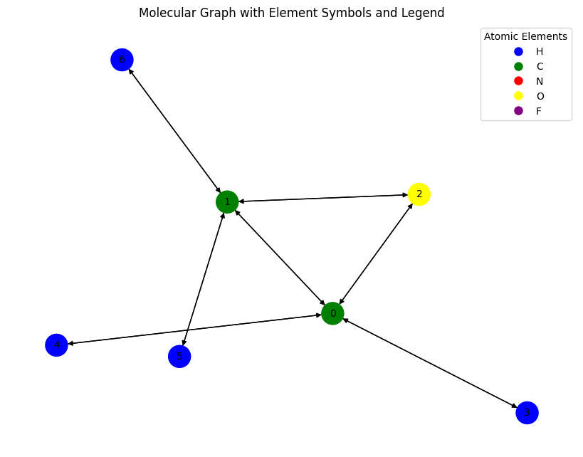
# Lets visualize a few samples
import networkx as nx
from torch_geometric.utils import to_networkx

# Convert the PyTorch Geometric graph to a NetworkX graph
G = to_networkx(data, node_attrs=['x'], edge_attrs=None)

# Inspect the graph
print(G.nodes(data=True))
print(G.edges(data=False))

[(0, {'x': [0.0, 1.0, 0.0, 0.0, 0.0, 6.0, 0.0, 0.0, 0.0, 0.0, 2.0]}), (1, {'x': [0.0, 1.0, 0.0, 0.0, 0.0, 6.0, 0.0, 0.0, 0.0, 0.0, 2.0]}), (2, {'x': [0.0, 0.0, 0.0, 1.0, 0.0, 8.0, 0.0, 0.0, 0.0, 0.0, 0.0]}), (3, {'x': [1.0, 0.0, 0.0, 0.0, 0.0, 1.0, 0.0, 0.0, 0.0, 0.0, 0.0]}), (4, {'x': [1.0, 0.0, 0.0, 0.0, 0.0, 1.0, 0.0, 0.0, 0.0, 0.0, 0.0]}), (5, {'x': [1.0, 0.0, 0.0, 0.0, 0.0, 1.0, 0.0, 0.0, 0.0, 0.0, 0.0]}), (6, {'x': [1.0, 0.0, 0.0, 0.0, 0.0, 1.0, 0.0, 0.0, 0.0, 0.0, 0.0]})]
[(0, 1), (0, 2), (0, 3), (0, 4), (1, 0), (1, 2), (1, 5), (1, 6), (2, 0), (2, 1), (3, 0), (4, 0), (5, 1), (6, 1)]

# Mapping atomic numbers to elements and colors
atomic_number_to_element = {1: 'H', 6: 'C', 7: 'N', 8: 'O', 9: 'F'}
atomic_number_to_color = {1: 'blue', 6: 'green', 7: 'red', 8: 'yellow', 9: 'purple'}

for (atomic_number, color), (_, element) in zip(atomic_number_to_color.items(), atomic_number_to_element.items()):
  print(f"atomic_number: {atomic_number}, element: {element}, color: {color}")

atomic_number: 1, element: H, color: blue
atomic_number: 6, element: C, color: green
atomic_number: 7, element: N, color: red
atomic_number: 8, element: O, color: yellow
atomic_number: 9, element: F, color: purple

from torch_geometric.utils import to_networkx
import matplotlib.pyplot as plt
import networkx as nx


# Convert PyTorch Geometric graph to NetworkX
G = to_networkx(data)

# Extract atomic numbers and corresponding elements/colors
atomic_numbers = data.x[:, 5].tolist()  # Assuming column 5 contains atomic numbers
elements = [atomic_number_to_element[int(z)] for z in atomic_numbers]
node_colors = [atomic_number_to_color[int(z)] for z in atomic_numbers]

# Create a legend
legend_elements = [
    plt.Line2D([0], [0], marker='o', color='w', markerfacecolor=color, markersize=10, label=atomic_number_to_element[atomic_number])
    for atomic_number, color in atomic_number_to_color.items()
]

# Node labels using element symbols
node_labels = {i: elements[i] for i in range(len(elements))}

# Plot the graph
plt.figure(figsize=(8, 6))
nx.draw(
    G,
    #labels=node_labels,
    with_labels=True,
    node_color=node_colors,
    edge_color='black',
    node_size=500,
    font_size=10,
    arrows=True  # This shows direction if G is a DiGraph
)

# Add the legend
plt.legend(handles=legend_elements, loc='best', title="Atomic Elements")
plt.title("Molecular Graph with Element Symbols and Legend")
plt.show()

_images/2c8a362d8c17b02d7302464b27cee47f08ab381cd8fd366d042a4174edda3ee8.png

# New information can be added as

data.new_attribute = torch.tensor([1, 2, 3])
data

Data(x=[7, 11], edge_index=[2, 14], edge_attr=[14, 4], y=[1, 19], pos=[7, 3], idx=[1], name='gdb_17', z=[7], new_attribute=[3])

data.edge_index

tensor([[0, 0, 0, 0, 1, 1, 1, 1, 2, 2, 3, 4, 5, 6],
        [1, 2, 3, 4, 0, 2, 5, 6, 0, 1, 0, 0, 1, 1]])

# Remove last edge and its attr
data.edge_index = data.edge_index[:, :-1]
data.edge_attr = data.edge_attr[:-1]

data

Data(x=[7, 11], edge_index=[2, 13], edge_attr=[13, 4], y=[1, 19], pos=[7, 3], idx=[1], name='gdb_17', z=[7], new_attribute=[3])

# Convert PyTorch Geometric graph to NetworkX
Gnew = to_networkx(data)

# Plot the new graph
plt.figure(figsize=(8, 6))
nx.draw(
    Gnew,
    #labels=node_labels,
    with_labels=True,
    node_color=node_colors,
    edge_color='black',
    node_size=500,
    font_size=10,
    arrows=True  # This shows direction if G is a DiGraph
)

# Add the legend
plt.legend(handles=legend_elements, loc='best', title="Atomic Elements")
plt.title("Molecular Graph with Element Symbols and Legend")
plt.show()

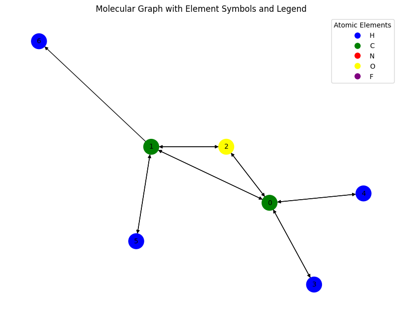
_images/fca1dbefe339b6e289140e5464a5b8e6c6713c402660f69f32ef902dbdd79ede.png

😀 notice the difference between the two graphs?

device = torch.device("cuda:0" if torch.cuda.is_available() else "cpu")
data.to(device)
data.new_attribute.is_cuda # check if new_attribute is part of data and seen by device

True

28.4. NNConv: Neural Message Passing Convolution#

The NNConv layer in torch_geometric.nn implements a continuous kernel-based convolution operator as introduced in the Neural Message Passing for Quantum Chemistry paper.

This layer is particularly designed for graph-structured data where the edges contain important information, such as molecular bonds or other edge features.

28.4.1. 🔍 How it works#

NNConv generalizes the message passing framework by learning edge-conditioned filters:

\[ \mathbf{x}_i' = \Theta \mathbf{x}_i + \sum_{j \in \mathcal{N}(i)} \mathbf{x}_j \cdot h_{\theta}(e_{i,j}) \]

\(\mathbf{x}_i\): Feature vector of node \(i\)
\(\mathcal{N}(i)\): Neighborhood of node \(i\)
\(e_{i,j}\): Edge features between node \(i\) and \(j\)
\(h_{\theta}\): Neural network applied to edge features to generate convolution weights; it maps edge features [-1, num_edge_features] to shape [-1, in_channels * out_channels], e.g., defined by torch.nn.Sequential.
\(\Theta\): Learnable transformation for self-node feature

28.4.2. Parameters#

NNConv(
    in_channels,        # Input feature dimension
    out_channels,       # Output feature dimension
    nn,                 # A neural network mapping edge features to weight matrices
    aggr='add',         # Aggregation method: 'add', 'mean', or 'max'
    root_weight=True,   # Whether to add a root transformation (Θ)
    bias=True           # Include bias term
)

28.5. Edge-Conditioned Learning with NNConv#

This notebook demonstrates a graph neural network (GNN) model using edge-conditioned convolutions. It’s particularly useful for tasks like molecular property prediction, where both node features (e.g., atom types) and edge features (e.g., bond types, bond lengths) carry important information.

28.5.1. 🤔 What is NNConv? Is it a GCN?#

GCN (Kipf & Welling) uses fixed weights shared across all edges — it doesn’t use edge features.
NNConv is a generalization of GCN, where each edge can have its own learnable weight matrix. These are computed dynamically from edge features via a neural network.
This makes NNConv a message-passing GNN layer — still a type of graph convolution, but edge-aware and more expressive.

28.5.2. Tensor Shapes#

Symbol	Meaning
`N`	Number of nodes
`E`	Number of edges
`F_in`	Input features per node
`F_edge`	Input features per edge
`B`	Batch size (number of graphs)

28.5.3. Model Architecture#

This GNN does the following:

Inputs: Node features and edge features.
GNN Layers: Two NNConv layers with neural networks to learn edge-conditioned weights.
Graph Pooling: Use global_add_pool to aggregate node features into a single graph-level representation.
Output: A scalar per graph, useful for regression tasks like predicting molecular energy.

28.5.4. Why Edge-Conditioned?#

Edge-conditioned learning allows message transformations to depend on edge-specific properties — such as bond types or lengths in a molecule. This results in more expressive models compared to traditional GCNs that ignore edge attributes.

#############################################################################################################
# Below an example of how to build a message passing network using PyTorch Geometric using the NNConv layer #
#############################################################################################################



class ExampleNet(torch.nn.Module):
    def __init__(self,num_node_features,num_edge_features):
        super().__init__()

        # Remember:
        # x: Node features — shape [N, F_in]
        # edge_index: Graph connectivity — shape [2, E]
        # edge_attr: Edge features — shape [E, F_edge]

        # The following are edge-aware layers
        conv1_net = nn.Sequential(nn.Linear(num_edge_features, 32),    # [E, F_edge] → [E, 32]
                                  nn.ReLU(),
                                  nn.Linear(32, num_node_features*32)) # [E, 32] → [E, F_in*32] --- So each edge generates a [F_in × 32] transformation matrix
                                  # N.b.: you don’t want an activation at the end: adding ReLU would restrict the weight matrix to non-negative values, which limits expressivity
        # Output shape before reshaping: [E, F_in * 32]
        # Reshaped by NNConv internally to: [E, F_in, 32]

        conv2_net = nn.Sequential(nn.Linear(num_edge_features,32),     # [E, F_edge] → [E, 32]
                                  nn.ReLU(),
                                  nn.Linear(32, 32*16))                # [E, 32] → [E, 32 * 16]
        # Output shape before reshaping: [E, 32 * 16]
        # Reshaped by NNConv internally to: [E, 32, 16]

        # Can you extend to a "3rd layer"?

        self.conv1 = NNConv(num_node_features, 32, conv1_net)
        # Input:
        #   x: [N, F_in]
        #   edge_attr: [E, F_edge]
        # Output:
        #   x: [N, 32]

        # Takes x from conv1
        self.conv2 = NNConv(32, 16, conv2_net)
        # Input:
        #   x: [N, 32]
        #   edge_attr: [E, F_edge]
        # Output:
        #   x: [N, 16]

        # N.B.: The more layers you stack, the further information can flow in the graph...
        # After 1 GNN layer (e.g., conv1), each node’s features are updated using its immediate neighbors' features.
        # After 2 layers, each node has aggregated information from its neighbors and their neighbors (2-hop neighborhood)...

        ############################ Can you extend to a "3rd layer"? ###############################

        self.fc_1 = nn.Linear(16, 32)

        self.out = nn.Linear(32, 1)

    def forward(self, data):
        batch, x, edge_index, edge_attr=data.batch, data.x, data.edge_index, data.edge_attr

        # batch = data.batch               # Shape: [N], maps each node to a graph in batch
        # x = data.x                       # Shape: [N, F_in]
        # edge_index = data.edge_index     # Shape: [2, E]
        # edge_attr = data.edge_attr       # Shape: [E, F_edge]


        # edge_weight_matrices = conv1_net(edge_attr) # [E, F_edge] -> [E, F_in * 32] reshaped [E, F_in, 32]
        # For each edge e, this gives a unique weight matrix W_e of shape [F_in, 32].
        #
        #   What does NNconv do?
        #   0. Compute the weights = conv1_net(edge_attr)  # shape: [E, F_in * 32]
        #   1. Fetch the feature vector x_j of the source node j: shape [F_in]
        #   2. Multiply it by the edge-specific matrix W_e: W_e @ x_j  →  [F_in, 32] @ [F_in] = shape [32]
        #   3. Aggregate messages at each target node i: x_i_new = sum_{j in N(i)} W_ij @ x_j = shape [32]
        #   Do this for all aggregated output: shape [N, 32]


        x = F.relu(self.conv1(x, edge_index, edge_attr))
        # input
        #   x : [N, F_in]
        #   edge_attr: [E, F_edge]
        # Output: [N, 32]

        x = F.relu(self.conv2(x, edge_index, edge_attr))
        #   x : [N, 32]
        #   edge_attr: [E, F_edge]
        # Output: [N, 16]


        x = global_add_pool(x,batch)
        # Input:
        #   x: [N, 16]
        #   batch: [N]  → tells which of B graphs each node belongs to
        # Output: [B, 16]

        x = F.relu(self.fc_1(x)) # [B, 16] → [B, 32]
        output = self.out(x)     # [B, 32] → [B, 1]

        return output

from torch.utils.data import random_split


train_set, valid_set, test_set = random_split(dset,[110000, 10831, 10000])

trainloader = DataLoader(train_set, batch_size=32, shuffle=True)
validloader = DataLoader(valid_set, batch_size=32, shuffle=True)
testloader = DataLoader(test_set, batch_size=32, shuffle=True)

qm9_node_feats, qm9_edge_feats = 11, 4
net = ExampleNet(qm9_node_feats, qm9_edge_feats)

optimizer = torch.optim.Adam(net.parameters(), lr=0.01)
target_idx = 1 # index position of the polarizability label

device = torch.device("cuda:0" if torch.cuda.is_available() else "cpu")
net.to(device)

ExampleNet(
  (conv1): NNConv(11, 32, aggr=add, nn=Sequential(
    (0): Linear(in_features=4, out_features=32, bias=True)
    (1): ReLU()
    (2): Linear(in_features=32, out_features=352, bias=True)
  ))
  (conv2): NNConv(32, 16, aggr=add, nn=Sequential(
    (0): Linear(in_features=4, out_features=32, bias=True)
    (1): ReLU()
    (2): Linear(in_features=32, out_features=512, bias=True)
  ))
  (fc_1): Linear(in_features=16, out_features=32, bias=True)
  (out): Linear(in_features=32, out_features=1, bias=True)
)

epochs = 10

train_loss_list = []
valid_loss_list = []


for total_epochs in range(epochs):

    train_loss = 0
    total_graphs = 0
    net.train()
    for batch in trainloader:
        batch.to(device)
        optimizer.zero_grad()
        output = net(batch)
        loss = F.mse_loss(output, batch.y[:, target_idx].unsqueeze(1)) #[num_graphs] -> [num_graphs,1]
        loss.backward()
        train_loss += loss.item()
        total_graphs += batch.num_graphs  #internally defined in torch_geometric.data.Batch
        optimizer.step()

    train_avg_loss = train_loss / total_graphs

    val_loss = 0
    total_graphs = 0
    net.eval()
    for batch in validloader:
        batch.to(device)
        output = net(batch)
        loss = F.mse_loss(output,batch.y[:, target_idx].unsqueeze(1))
        val_loss += loss.item()
        total_graphs += batch.num_graphs

    val_avg_loss = val_loss / total_graphs


    print(f"Epochs: {total_epochs} | training avg. loss: {train_avg_loss:.3f} | validation avg. loss: {val_avg_loss:.3f}")
    train_loss_list.append(train_avg_loss)
    valid_loss_list.append(val_avg_loss)

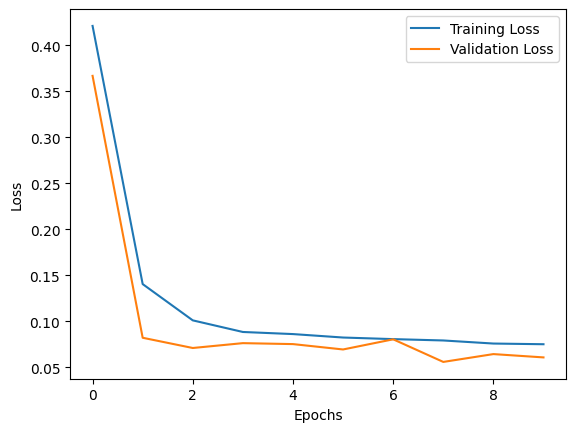
Epochs: 0 | training avg. loss: 0.421 | validation avg. loss: 0.367
Epochs: 1 | training avg. loss: 0.141 | validation avg. loss: 0.082
Epochs: 2 | training avg. loss: 0.101 | validation avg. loss: 0.071
Epochs: 3 | training avg. loss: 0.088 | validation avg. loss: 0.076
Epochs: 4 | training avg. loss: 0.086 | validation avg. loss: 0.075
Epochs: 5 | training avg. loss: 0.082 | validation avg. loss: 0.069
Epochs: 6 | training avg. loss: 0.081 | validation avg. loss: 0.081
Epochs: 7 | training avg. loss: 0.079 | validation avg. loss: 0.056
Epochs: 8 | training avg. loss: 0.076 | validation avg. loss: 0.064
Epochs: 9 | training avg. loss: 0.075 | validation avg. loss: 0.061

plt.plot(train_loss_list, label='Training Loss')
plt.plot(valid_loss_list, label='Validation Loss')
plt.xlabel('Epochs')
plt.ylabel('Loss')
plt.legend()
plt.show()

_images/b06fabb3b02881d65311e0610497514fe5158330b52f7d0b8567063423c3735c.png

net.eval() # model in evaluation mode; Disables things like Dropout and BatchNorm updates; does not disable gradient tracking
predictions = []
real = []

for batch in testloader:

    output = net(batch.to(device))
    predictions.append(output.detach().cpu().numpy())
    real.append(batch.y[:, target_idx].detach().cpu().numpy())

predictions = np.concatenate(predictions)
real = np.concatenate(real)

import matplotlib.pyplot as plt


plt.scatter(real[:2000],predictions[:2000])
plt.ylabel('Predicted isotropic polarizability')
plt.xlabel('Isotropic polarizability')
plt.xlim(20,120)
plt.ylim(20,120)
# display as square
plt.gca().set_aspect('equal', adjustable='box')
plt.show()

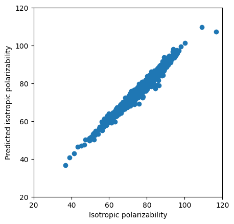
_images/81d4c03af5c9fb799bd0b6da393ca06afbe6ed9f5f8d31f38256a2652996387b.png

from sklearn.metrics import r2_score

r2 = r2_score(real[:2000], predictions[:2000])
print(f"R² Score: {r2:.4f}")

R² Score: 0.9741

28.6. Extension to Multiple Layers#

Exercise: Let’s extend the previous problem to three layers.

28.7. The Non Edge-Aware Case#

######################################################################################
# Below an example of how to build a message passing network which is not edge-aware #
######################################################################################

import torch
import torch.nn.functional as F
from torch_geometric.nn import GCNConv, global_add_pool

class ExampleGCN(torch.nn.Module):
    def __init__(self, num_node_features):
        super().__init__()

        # No edge_attr needed!
        # https://pytorch-geometric.readthedocs.io/en/2.5.2/generated/torch_geometric.nn.conv.GCNConv.html
        self.conv1 = GCNConv(num_node_features, 32)
        self.conv2 = GCNConv(32, 16)
        self.conv3 = GCNConv(16, 8)

        self.fc_1 = torch.nn.Linear(8, 32)
        self.out = torch.nn.Linear(32, 1)

    def forward(self, data):
        x, edge_index, batch = data.x, data.edge_index, data.batch

        x = F.relu(self.conv1(x, edge_index))   # [N, F_in] → [N, 32]
        x = F.relu(self.conv2(x, edge_index))   # [N, 32] → [N, 16]
        x = F.relu(self.conv3(x, edge_index))   # [N, 16] → [N, 8]

        x = global_add_pool(x, batch)           # [N, 8] → [B, 8]
        x = F.relu(self.fc_1(x))                # [B, 8] → [B, 32]
        output = self.out(x)                    # [B, 32] → [B, 1]

        return output

qm9_node_feats = 11

net_gcn = ExampleGCN(qm9_node_feats)

optimizer = torch.optim.Adam(net_gcn.parameters(), lr=0.01)
target_idx = 1 # index position of the polarizability label

device = torch.device("cuda:0" if torch.cuda.is_available() else "cpu")
net_gcn.to(device)

ExampleGCN(
  (conv1): GCNConv(11, 32)
  (conv2): GCNConv(32, 16)
  (conv3): GCNConv(16, 8)
  (fc_1): Linear(in_features=8, out_features=32, bias=True)
  (out): Linear(in_features=32, out_features=1, bias=True)
)

train_loss_list = []
valid_loss_list = []

for total_epochs in range(epochs):

    train_loss = 0
    total_graphs = 0
    net.train()
    for batch in trainloader:
        batch.to(device)
        optimizer.zero_grad()
        output = net_gcn(batch)
        loss = F.mse_loss(output, batch.y[:, target_idx].unsqueeze(1))
        loss.backward()
        train_loss += loss.item()
        total_graphs += batch.num_graphs
        optimizer.step()

    train_avg_loss = train_loss / total_graphs

    val_loss = 0
    total_graphs = 0
    net.eval()
    for batch in validloader:
        batch.to(device)
        output = net_gcn(batch)
        loss = F.mse_loss(output,batch.y[:, target_idx].unsqueeze(1))
        val_loss += loss.item()
        total_graphs += batch.num_graphs
    val_avg_loss = val_loss / total_graphs


    print(f"Epochs: {total_epochs} | train avg. loss: {train_avg_loss:.2f} | validation avg. loss: {val_avg_loss:.2f}")
    train_loss_list.append(train_avg_loss)
    valid_loss_list.append(val_avg_loss)

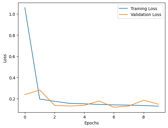
Epochs: 0 | train avg. loss: 1.06 | validation avg. loss: 0.24
Epochs: 1 | train avg. loss: 0.20 | validation avg. loss: 0.28
Epochs: 2 | train avg. loss: 0.18 | validation avg. loss: 0.14
Epochs: 3 | train avg. loss: 0.16 | validation avg. loss: 0.13
Epochs: 4 | train avg. loss: 0.15 | validation avg. loss: 0.14
Epochs: 5 | train avg. loss: 0.15 | validation avg. loss: 0.18
Epochs: 6 | train avg. loss: 0.14 | validation avg. loss: 0.12
Epochs: 7 | train avg. loss: 0.14 | validation avg. loss: 0.13
Epochs: 8 | train avg. loss: 0.14 | validation avg. loss: 0.19
Epochs: 9 | train avg. loss: 0.13 | validation avg. loss: 0.15

plt.plot(train_loss_list, label='Training Loss')
plt.plot(valid_loss_list, label='Validation Loss')
plt.xlabel('Epochs')
plt.ylabel('Loss')
plt.legend()
plt.show()

_images/44feaff96a8b93c5de03fd434f8e2a2d272512a90e6a2acdb0350c308ca4733a.png

net_gcn.eval() # model in evaluation mode; Disables things like Dropout and BatchNorm updates; does not disable gradient tracking
predictions = []
real = []

for batch in testloader:

    output = net_gcn(batch.to(device))
    predictions.append(output.detach().cpu().numpy())
    real.append(batch.y[:, target_idx].detach().cpu().numpy())

predictions = np.concatenate(predictions)
real = np.concatenate(real)

plt.scatter(real[:2000],predictions[:2000])
plt.ylabel('Predicted isotropic polarizability')
plt.xlabel('Isotropic polarizability')
plt.xlim(20,120)
plt.ylim(20,120)
# display as square
plt.gca().set_aspect('equal', adjustable='box')
plt.show()

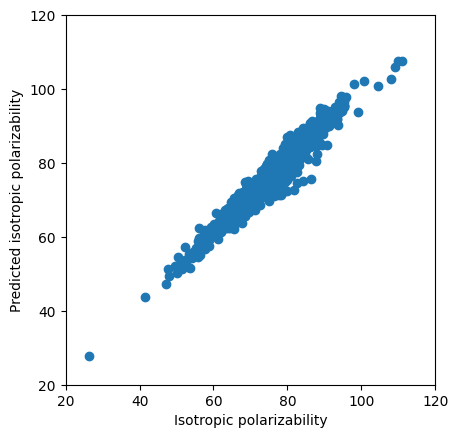
_images/fa928c616123e54842dec055c360989ec57d77704dc576050475df553d47edc0.png

r2 = r2_score(real[:2000], predictions[:2000])
print(f"R² Score: {r2:.4f}")

R² Score: 0.9379