
Credits: Raschka et al., Chap 14
18. Convolutional Neural Network - Part 1#
from IPython.display import Image
from IPython.display import display
%matplotlib inline
Outline
18.1. The building blocks of convolutional neural networks#
CNN inspired by the functioning of the visual cortex in our brain. Experiment in 1959 with an anesthetized cat. Neurons respond differently after projecting different patterns of light in front of the cat. Primary layers of the viual cortex detects edges and straight lines, highger order layers focus more on extracting complex shapes.
In CNN, early layers extract low-level features from the raw data, later layers (often fully connected as in MLP) use these features to predict a target value.
CNN typically perform well on image data.
In Fig. 1, you see how to create feature maps from an image. The local patch of pixels is referred to as local receptive field.
# FIG 1
display(Image(url="https://raw.githubusercontent.com/cfteach/NNDL_DATA621/webpage-src/DATA621/DATA621/images/Fig1_lec10.png", height=200))

CNN performs well on image-related tasks largely due to two ideas:
Sparse connectivity: A single element in the feature map (output of the convolutional layer) is connected to only a small patch of pixels. This is very different from MLP (connections to the whole image).
Parameter sharing: The same weights are used for different patches of the input image using the same filter.
CNN made of following layers:
convolutional -> have learnable parameters
subsampling -> no learnable parameters
fully connected -> have learnable parameters
18.2. Performing discrete convolutions#
Convolution applies a small filter (kernel) over the input x, allowing it to detect local structures like edges, textures, and patterns.
Discrete convolutions in one dimension
https://en.wikipedia.org/wiki/Convolution
We want to achieve this through a filter (w) :
Before applying the above, first thing we might need to do is padding.
# FIG 2
display(Image(url="https://raw.githubusercontent.com/cfteach/NNDL_DATA621/webpage-src/DATA621/DATA621/images/Fig2_lec10.png", width=600))

Then, after padding, you can calculate the convolution this way:
# FIG 3
display(Image(url="https://raw.githubusercontent.com/cfteach/NNDL_DATA621/webpage-src/DATA621/DATA621/images/Fig3_lec10.png", width=600))
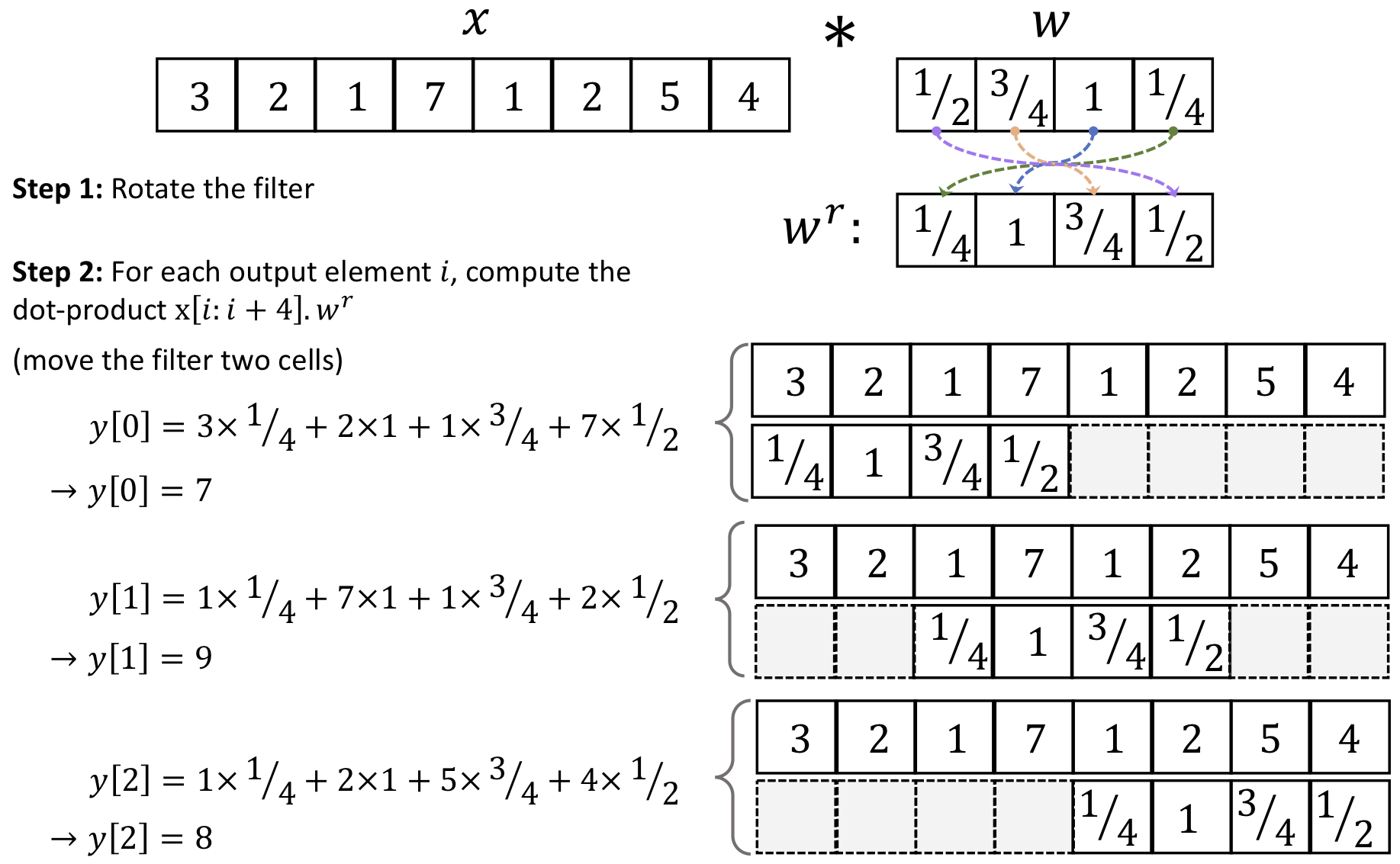
Okay, one thing at the time. Let’s take a look at padding first.
18.3. Padding inputs to control the size of the output feature maps#
Why Padding Matters?
Prevents excessive shrinking of feature maps in deep networks.
Controls how much context the kernel sees near the edges.
Balances computational efficiency vs. accuracy.
1. Full Padding
Adds the most padding (zero-padding around the input).
The output is larger than the input.
Ensures that the kernel has a valid position even at the edges.
2. Same Padding (Most common in CNNs)
Adds just enough padding so that the output size remains the same as the input size (assuming stride = 1).
This helps preserve spatial dimensions throughout the layers.
3. Valid Padding (No Padding)
No padding is added, meaning the kernel only moves over the valid input positions.
The output is smaller than the input.
# FIG 4
display(Image(url="https://raw.githubusercontent.com/cfteach/NNDL_DATA621/webpage-src/DATA621/DATA621/images/Fig4_lec10.png", width=600))

18.4. Determining the size of the convolution output#
An important formula to remember is
which gives the convolution output
import torch
import numpy as np

print('PyTorch version:', torch.__version__)
print('NumPy version: ', np.__version__)
PyTorch version: 2.5.1+cu124
NumPy version:  1.26.4
Some gym… 😴 ⏰
w = [1, 0, 3, 1, 2]
w[: :-1]
[2, 1, 3, 0, 1]
w = np.zeros((4,5))
np.shape(w)
(4, 5)
w[2,3]=-17
w[1,2]=3.
w[3,1] =2.
w
array([[  0.,   0.,   0.,   0.,   0.],
       [  0.,   0.,   3.,   0.,   0.],
       [  0.,   0.,   0., -17.,   0.],
       [  0.,   2.,   0.,   0.,   0.]])
w[: : -2]
array([[0., 2., 0., 0., 0.],
       [0., 0., 3., 0., 0.]])
w[: :]
array([[  0.,   0.,   0.,   0.,   0.],
       [  0.,   0.,   3.,   0.,   0.],
       [  0.,   0.,   0., -17.,   0.],
       [  0.,   2.,   0.,   0.,   0.]])
w = [1, 0, 3, 1, 2]
w[: : -1]
[2, 1, 3, 0, 1]
## 1D convolutional

def conv1d(x, w, p=0, s=1):
    w_rot = np.array(w[::-1])
    x_padded = np.array(x)
    if p > 0:
        zero_pad = np.zeros(shape=p)
        x_padded = np.concatenate(
            [zero_pad, x_padded, zero_pad])
    res = []
    for i in range(0, (int((len(x_padded) - len(w_rot))/s) + 1), s):
        res.append(np.sum(
            x_padded[i:i + w_rot.shape[0]] * w_rot))
    return np.array(res)


## Testing:
x = [1, 3, 2, 4, 5, 6, 1, 3]
w = [1, 0, 3, 1, 2]

print(np.array(w[::-1]))
print(np.shape(np.array(w[::-1])))
print(np.array(w[::-1]).shape[0])

print('Conv1d Implementation:',
      conv1d(x, w, p=2, s=1))

print('Numpy Results:',
      np.convolve(x, w, mode='same'))
[2 1 3 0 1]
(5,)
5
Conv1d Implementation: [ 5. 14. 16. 26. 24. 34. 19. 22.]
Numpy Results: [ 5 14 16 26 24 34 19 22]
w = np.zeros((3,3))
w[1,2]=-1.
w[0,1]=3.
w[2,1]=2.
print(w)
[[ 0.  3.  0.]
 [ 0.  0. -1.]
 [ 0.  2.  0.]]
w[::-1]
array([[ 0.,  2.,  0.],
       [ 0.,  0., -1.],
       [ 0.,  3.,  0.]])
w[::-1, ::-1] # "180 degree operation"
array([[ 0.,  2.,  0.],
       [-1.,  0.,  0.],
       [ 0.,  3.,  0.]])
18.5. Performing a discrete convolution in 2D#
# FIG 5
display(Image(url="https://raw.githubusercontent.com/cfteach/NNDL_DATA621/webpage-src/DATA621/DATA621/images/Fig5_lec10.png", width=600))

Suppose you want to do this convolution
# conv 2d
display(Image(url="https://raw.githubusercontent.com/cfteach/NNDL_DATA621/webpage-src/DATA621/DATA621/images/conv2d_lec10.png", width=600))
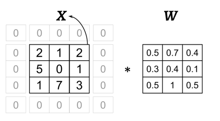
Consider the following image: what values of p, m and s have been used in the convolution?
# FIG 6
display(Image(url="https://raw.githubusercontent.com/cfteach/NNDL_DATA621/webpage-src/DATA621/DATA621/images/Fig6_lec10.png", width=600))

p=(0, 0)
X_orig = np.zeros((3,3))
n1 = X_orig.shape[0] + 2*p[0]
n2 = X_orig.shape[1] + 2*p[1]

print(n1, n2)
3 3
import scipy.signal


def conv2d(X, W, p=(0, 0), s=(1, 1)):
    W_rot = np.array(W)[::-1,::-1]
    X_orig = np.array(X)
    n1 = X_orig.shape[0] + 2*p[0]
    n2 = X_orig.shape[1] + 2*p[1]
    X_padded = np.zeros(shape=(n1, n2))
    X_padded[p[0]:p[0]+X_orig.shape[0],
    p[1]:p[1]+X_orig.shape[1]] = X_orig

    print(W_rot)

    res = []
    for i in range(0, (int((X_padded.shape[0] -
                            W_rot.shape[0]) / s[0]) + 1), s[0]):
        res.append([])
        for j in range(0, (int((X_padded.shape[1] -
                                W_rot.shape[1]) / s[1]) + 1), s[1]):
            X_sub = X_padded[i:i + W_rot.shape[0],
                    j:j + W_rot.shape[1]]
            res[-1].append(np.sum(X_sub * W_rot))
    return(np.array(res))

X = [[1, 3, 2, 4], [5, 6, 1, 3], [1, 2, 0, 2], [3, 4, 3, 2]]
W = [[1, 0, 3], [1, 2, 1], [0, 1, 1]]

print('Conv2d Implementation:\n',
    conv2d(X, W, p=(1, 1), s=(1, 1)))


print('SciPy Results:\n',
    scipy.signal.convolve2d(X, W, mode='same'))
[[1 1 0]
 [1 2 1]
 [3 0 1]]
Conv2d Implementation:
 [[11. 25. 32. 13.]
 [19. 25. 24. 13.]
 [13. 28. 25. 17.]
 [11. 17. 14.  9.]]
SciPy Results:
 [[11 25 32 13]
 [19 25 24 13]
 [13 28 25 17]
 [11 17 14  9]]
18.6. Subsampling layers#
# FIG 7
display(Image(url="https://raw.githubusercontent.com/cfteach/NNDL_DATA621/webpage-src/DATA621/DATA621/images/Fig7_lec10.png", height=250))

18.7. Putting everything together – implementing a CNN#
Working with multiple input or color channels
In the following example:
The input has 3 channels
Each filter has a depth of 3, matching the number of input channels.
The number of filters (C_out = 5) determines the number of output feature maps. Each filter produces one feature map, meaning the output has 5 feature maps.
A pooling operation (e.g., max pooling, average pooling) is applied. It reduces spatial dimensions while maintaining 5 feature maps
# FIG 8
display(Image(url="https://raw.githubusercontent.com/cfteach/NNDL_DATA621/webpage-src/DATA621/DATA621/images/Fig8_lec10.png", width=600))

18.8. The multilayer CNN architecture with PyTorch#
# FIG 10
display(Image(url="https://raw.githubusercontent.com/cfteach/NNDL_DATA621/webpage-src/DATA621/DATA621/images/Fig10_lec10.png", width=600))
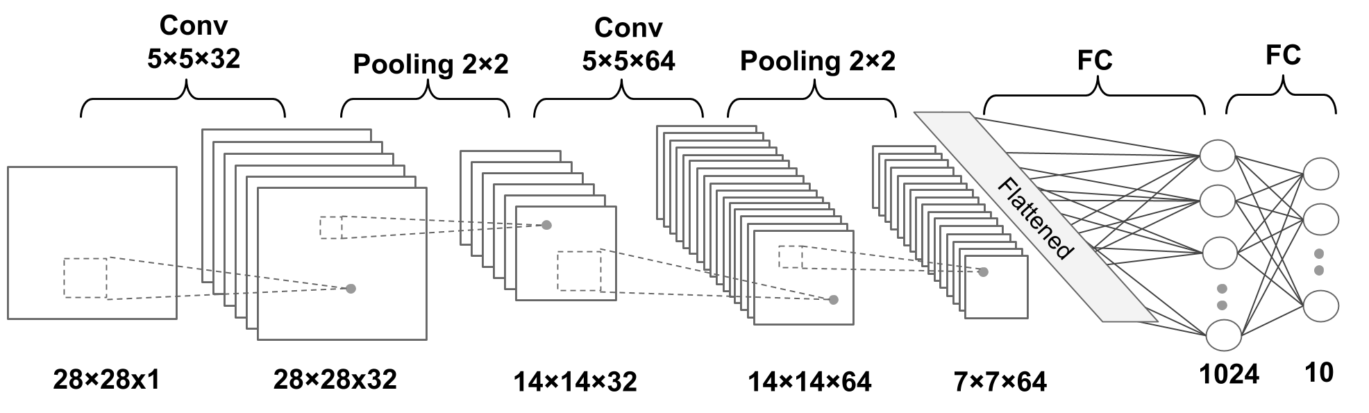
N.b.:
Convolution: default values of stride=1, padding=0 [https://pytorch.org/docs/stable/generated/torch.nn.Conv2d.html]
Pooling: default value of stride = kernel size [https://pytorch.org/docs/stable/generated/torch.nn.MaxPool2d.html]
18.8.1. Loading and preprocessing the data#
import numpy as np
import torch
import torch.nn as nn
#import torch.nn.functional as F
import torchvision
from torchvision import datasets
from torchvision import transforms
from torch.utils.data import DataLoader
device = torch.device("cuda" if torch.cuda.is_available() else "cpu")
print(device)

if device.type == 'cuda':
    print(torch.cuda.get_device_name(0))
else:
  print('cpu')
cuda
Tesla T4
image_path = './'  # see root=image_path, which specifies the directory where the dataset will be stored or loaded from.

# transforms.Compose is a function that composes several transforms together

# transforms.ToTensor() converts a PIL Image or numpy.ndarray (H x W x C) in the range [0, 255] to a torch.FloatTensor of shape (C x H x W) in the range [0.0, 1.0].
# In other words, if you apply transforms.ToTensor(), it automatically scales the values to the range [0, 1].
# This is necessary as PyTorch models expect inputs to be tensors.

transform = transforms.Compose([transforms.ToTensor()])

mnist_dataset = torchvision.datasets.MNIST(root=image_path,
                                           train=True, # the training set of the MNIST dataset is being requested.
                                           transform=transform, # transform=transform applies the transformation defined earlier
                                           download=True) # tells the library to download the dataset if it's not available at the specified root


from torch.utils.data import Subset

# create a validation subset
# torch.arange(10000) generates indices from 0 to 9999, selecting the first 10,000 samples from mnist_dataset to be used as validation
mnist_valid_dataset = Subset(mnist_dataset, torch.arange(10000))

# selects the remaining samples
mnist_train_dataset = Subset(mnist_dataset, torch.arange(10000, len(mnist_dataset)))

# the test set size is inherently predefined to be 10,000 images, no further specification is needed
mnist_test_dataset = torchvision.datasets.MNIST(root=image_path,
                                           train=False,
                                           transform=transform,
                                           download=False)

#---- please notice that mnist_test_dataset still require to be scaled, differently from mnist_train_dataset and mnist_valid_dataset
#---- see later
print(len(mnist_train_dataset),len(mnist_valid_dataset),len(mnist_test_dataset))

sample_image, sample_label = mnist_train_dataset[0]

print(sample_image.shape, sample_label)

# consistent NCHW format
50000 10000 10000
torch.Size([1, 28, 28]) 3
# We construct the data loader with batches of batch_size images for the training set and validation set

from torch.utils.data import DataLoader


batch_size = 64
torch.manual_seed(1)
train_dl = DataLoader(mnist_train_dataset, batch_size, shuffle=True)
valid_dl = DataLoader(mnist_valid_dataset, batch_size, shuffle=False) #Why?
for tmpbatch in train_dl:
  #print(type(tmpbatch))
  break
tmp_in = tmpbatch[0]
tmp_out = tmpbatch[1]

print(tmp_in.shape, tmp_out.shape)
torch.Size([64, 1, 28, 28]) torch.Size([64])
print(tmp_in.min())
tensor(0.)
18.8.2. Configuring CNN layers in PyTorch#
Conv2d:
torch.nn.Conv2dout_channelskernel_sizestridepadding
MaxPool2d:
torch.nn.MaxPool2dkernel_sizestridepadding
Dropout
torch.nn.Dropoutp
18.9. Constructing a CNN in PyTorch#
model = nn.Sequential()
model.add_module('conv1', nn.Conv2d(in_channels=1, out_channels=32, kernel_size=5, padding=2)) # A convolution operation is linear...
model.add_module('relu1', nn.ReLU())                  # The activation function makes the model non-linear, allowing it to learn more complex patterns...
model.add_module('pool1', nn.MaxPool2d(kernel_size=2)) #if stride=None, default is kernel_size
model.add_module('conv2', nn.Conv2d(in_channels=32, out_channels=64, kernel_size=5, padding=2))
model.add_module('relu2', nn.ReLU())
model.add_module('pool2', nn.MaxPool2d(kernel_size=2))
# PyTorch provides a convenient method to compute the size of the feature map for us

x = torch.ones((4, 1, 28, 28))
print(model(x).shape)
print(type(model(x).shape))

print(torch.prod(torch.tensor(model(x).shape)[1:]))
torch.Size([4, 64, 7, 7])
<class 'torch.Size'>
tensor(3136)
model.add_module('flatten', nn.Flatten())

x = torch.ones((4, 1, 28, 28))
model(x).shape
torch.Size([4, 3136])
Let’s add dropout
# FIG 9
display(Image(url="https://raw.githubusercontent.com/cfteach/NNDL_DATA621/webpage-src/DATA621/DATA621/images/Fig9_lec10.png", width=600))

model.add_module('fc1', nn.Linear(3136, 1024))
model.add_module('relu3', nn.ReLU())
model.add_module('dropout', nn.Dropout(p=0.5))

# --- Why dropout here?
# Earlier (e.g., right before relu3) application of dropout might lead to underfitting since ReLU turns all negative values to zero
# Dropout early in deep networks can severely limit the amount of learnable information,
# while dropout late in the network should be tuned to avoid overly damping the outputs (over-regularization).
# After ReLU and between (middle) layers.

model.add_module('fc2', nn.Linear(1024, 10))
device = torch.device("cuda:0")
#device = torch.device("cpu")

model = model.to(device)
loss_fn = nn.CrossEntropyLoss()
optimizer = torch.optim.Adam(model.parameters(), lr=0.001)
def train(model, num_epochs, train_dl, valid_dl):
loss_hist_train = [0] * num_epochs
accuracy_hist_train = [0] * num_epochs
loss_hist_valid = [0] * num_epochs
accuracy_hist_valid = [0] * num_epochs
for epoch in range(num_epochs):
#------ model.train() sets the model to training mode ------#
model.train()
for x_batch, y_batch in train_dl:
x_batch = x_batch.to(device)
y_batch = y_batch.to(device)
pred = model(x_batch)
loss = loss_fn(pred, y_batch)
#
loss.backward() # computes gradients
optimizer.step() # updates model parameters with gradients
optimizer.zero_grad() # resets all gradients to zero before the next backpropagation step
#
loss_hist_train[epoch] += loss.item()*y_batch.size(0) #loss.item() gives the average loss in the batch
is_correct = (torch.argmax(pred, dim=1) == y_batch).float()
accuracy_hist_train[epoch] += is_correct.sum().cpu()
loss_hist_train[epoch] /= len(train_dl.dataset)
accuracy_hist_train[epoch] /= len(train_dl.dataset)
#------ model.eval() sets the model to evaluation mode ------#
model.eval()
with torch.no_grad():
for x_batch, y_batch in valid_dl:
x_batch = x_batch.to(device)
y_batch = y_batch.to(device)
pred = model(x_batch)
loss = loss_fn(pred, y_batch)
loss_hist_valid[epoch] += loss.item()*y_batch.size(0)
is_correct = (torch.argmax(pred, dim=1) == y_batch).float()
accuracy_hist_valid[epoch] += is_correct.sum().cpu()
loss_hist_valid[epoch] /= len(valid_dl.dataset)
accuracy_hist_valid[epoch] /= len(valid_dl.dataset)
print(f'Epoch {epoch+1} accuracy: {accuracy_hist_train[epoch]:.4f} val_accuracy: {accuracy_hist_valid[epoch]:.4f}')
return loss_hist_train, loss_hist_valid, accuracy_hist_train, accuracy_hist_valid
torch.manual_seed(1)
num_epochs = 5
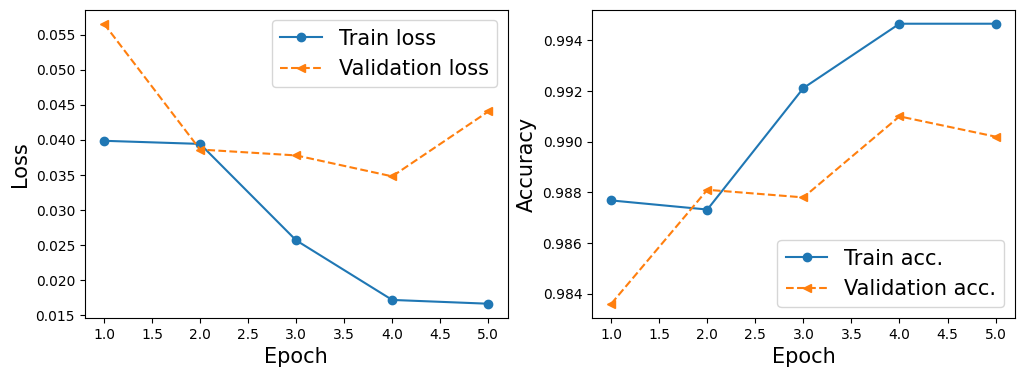
hist = train(model, num_epochs, train_dl, valid_dl)
Epoch 1 accuracy: 0.9877 val_accuracy: 0.9836
Epoch 2 accuracy: 0.9873 val_accuracy: 0.9881
Epoch 3 accuracy: 0.9921 val_accuracy: 0.9878
Epoch 4 accuracy: 0.9947 val_accuracy: 0.9910
Epoch 5 accuracy: 0.9947 val_accuracy: 0.9902
import matplotlib.pyplot as plt


x_arr = np.arange(len(hist[0])) + 1  # number of epochs

fig = plt.figure(figsize=(12, 4))

ax = fig.add_subplot(1, 2, 1)
ax.plot(x_arr, hist[0], '-o', label='Train loss')
ax.plot(x_arr, hist[1], '--<', label='Validation loss')
ax.set_xlabel('Epoch', size=15)
ax.set_ylabel('Loss', size=15)
ax.legend(fontsize=15)

ax = fig.add_subplot(1, 2, 2)
ax.plot(x_arr, hist[2], '-o', label='Train acc.')
ax.plot(x_arr, hist[3], '--<', label='Validation acc.')
ax.legend(fontsize=15)
ax.set_xlabel('Epoch', size=15)
ax.set_ylabel('Accuracy', size=15)

plt.show()
# cuda.synchronize()
# It is used to synchronize all CUDA operations.
# When you are running PyTorch on a GPU, operations are often asynchronous for efficiency.
# It ensures that all preceding CUDA operations are finished before moving on, important before switching from GPU to CPU.

torch.cuda.synchronize()

# moves the model from the GPU to the CPU.
model_cpu = model.cpu()


#pred = model(mnist_test_dataset.data.unsqueeze(1).float()) #.unsqueeze(1)/ 255.
pred = model(mnist_test_dataset.data.unsqueeze(1)/255.)

is_correct = (torch.argmax(pred, dim=1) == mnist_test_dataset.targets).float()
print(f'Test accuracy: {is_correct.mean():.4f}')
Test accuracy: 0.9899
print(mnist_test_dataset.data.shape)
print(mnist_test_dataset.data.unsqueeze(1).shape)
#mnist_test_dataset.data[0]
torch.Size([10000, 28, 28])
torch.Size([10000, 1, 28, 28])
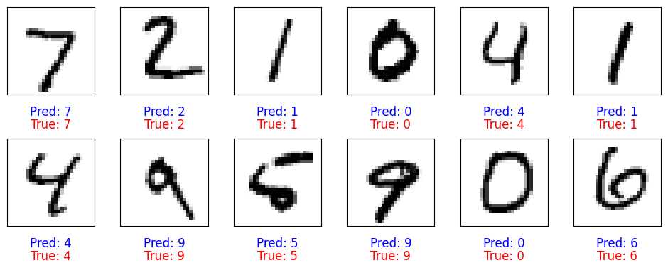
fig = plt.figure(figsize=(12, 4))
for i in range(12):
    ax = fig.add_subplot(2, 6, i+1)
    ax.set_xticks([]); ax.set_yticks([])
    img, true_label = mnist_test_dataset[i]
    img = img[0, :, :]  # Get the 2D image data from the tensor
    #img = mnist_test_dataset[i][0][0, :, :]   # mnist_test_dataset[i] contain image (tensor) and target (int)
    pred = model(img.unsqueeze(0).unsqueeze(1)) # unsqueeze adds a new dimension to a tensor at a specified position

    y_pred = torch.argmax(pred)
    ax.imshow(img, cmap='gray_r')

    # Add both predicted and ground truth labels to the plot
    ax.text(0.5, -0.2, f'Pred: {y_pred.item()}', size=12, color='blue',
            horizontalalignment='center', verticalalignment='center', transform=ax.transAxes)
    ax.text(0.5, -0.35, f'True: {true_label}', size=12, color='red',
            horizontalalignment='center', verticalalignment='center', transform=ax.transAxes)

# Adjust vertical spacing between rows (increase hspace)
plt.subplots_adjust(hspace=0.5)  # Increase space between rows (default is 0.2)


plt.show()
18.10. Randomly select an image, rotate, and make prediction#
import random
import torchvision.transforms.functional as TF

# Randomly select an image from the MNIST test dataset
random_idx = random.randint(0, len(mnist_test_dataset) - 1)  # Select a random index
img, true_label = mnist_test_dataset[random_idx]  # Get the image and true label
img = img.unsqueeze(0)  # Add batch dimension [1, 1, 28, 28]

# Rotate the image by a random angle
angle = random.uniform(-55, 55)  # Choose a random angle between -90 and 90 degrees
rotated_img = TF.rotate(img, angle)  # Rotate the image

# Make a prediction with the rotated image
pred = model(rotated_img)  # Run through the model
y_pred = torch.argmax(pred)  # Get the predicted label

# Plot the rotated image and show both the prediction and the true label
fig, ax = plt.subplots()
ax.set_xticks([]); ax.set_yticks([])

# Display the rotated image
ax.imshow(rotated_img.squeeze(), cmap='gray_r')

# Show predicted and true labels
ax.text(0.5, -0.1, f'Pred: {y_pred.item()}, True: {true_label}', size=15, color='blue',
        horizontalalignment='center', verticalalignment='center', transform=ax.transAxes)

plt.show()

print(f"angle: {angle:1.2f}")
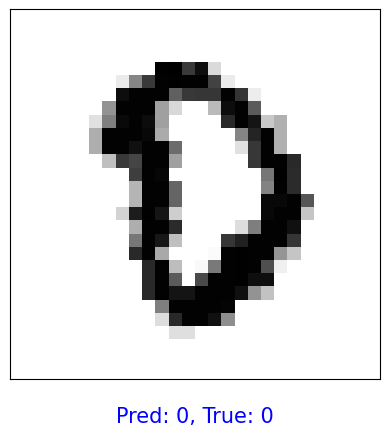
angle: 19.74
18.11. Add an extra convolutional layer#
Can you add to the prior model, before flattening, an extra convolutional layer 5x5x128? Please adjust the two FC layers to match the new dimensions.