(Tut 1) Deep Learning Deep Inelastic Scattering at EIC#

Credits:

Heavily based on:

Reconstructing the Kinematics of Deep Inelastic Scattering with Deep Learning by Miguel Arratia, Daniel Britzger, Owen Long, Benjamin Nachman arXiv:2110.05505 — [code, dataset]
Deeply Learning Deep Inelastic Scattering Kinematics, by Markus Diefenthaler, Abdullah Farhat, Andrii Verbytskyi, Yuesheng Xu,arXiv:2108.11638

Training for H1 rapgap MC with reconstructed observables as input.#

This uses a single DNN with all inputs (electron, HFS, photons)#

Adjust Huber delta to 0.01.

%load_ext autoreload
%autoreload 2

from google.colab import drive
drive.mount('/content/drive')

Mounted at /content/drive

# Make sure GPU runtime is enabled.
# Runtime -> Change Runtime Type -> Hardware Accelerator -> GPU
# You will likely only have a T4, unless you have colab pro.
!nvidia-smi

Wed Jun 21 22:06:09 2023       
+-----------------------------------------------------------------------------+
| NVIDIA-SMI 525.85.12    Driver Version: 525.85.12    CUDA Version: 12.0     |
|-------------------------------+----------------------+----------------------+
| GPU  Name        Persistence-M| Bus-Id        Disp.A | Volatile Uncorr. ECC |
| Fan  Temp  Perf  Pwr:Usage/Cap|         Memory-Usage | GPU-Util  Compute M. |
|                               |                      |               MIG M. |
|===============================+======================+======================|
|   0  Tesla T4            Off  | 00000000:00:04.0 Off |                    0 |
| N/A   52C    P8    12W /  70W |      0MiB / 15360MiB |      0%      Default |
|                               |                      |                  N/A |
+-------------------------------+----------------------+----------------------+
                                                                               
+-----------------------------------------------------------------------------+
| Processes:                                                                  |
|  GPU   GI   CI        PID   Type   Process name                  GPU Memory |
|        ID   ID                                                   Usage      |
|=============================================================================|
|  No running processes found                                                 |
+-----------------------------------------------------------------------------+

# We need uproot3 to unpack the ROOT file.
!pip install uproot3

Looking in indexes: https://pypi.org/simple, https://us-python.pkg.dev/colab-wheels/public/simple/
Collecting uproot3
  Downloading uproot3-3.14.4-py3-none-any.whl (117 kB)
     ━━━━━━━━━━━━━━━━━━━━━━━━━━━━━━━━━━━━━━━ 117.5/117.5 kB 4.4 MB/s eta 0:00:00
?25hRequirement already satisfied: numpy>=1.13.1 in /usr/local/lib/python3.10/dist-packages (from uproot3) (1.22.4)
Collecting awkward0 (from uproot3)
  Downloading awkward0-0.15.5-py3-none-any.whl (87 kB)
     ━━━━━━━━━━━━━━━━━━━━━━━━━━━━━━━━━━━━━━━━ 87.6/87.6 kB 10.5 MB/s eta 0:00:00
?25hCollecting uproot3-methods (from uproot3)
  Downloading uproot3_methods-0.10.1-py3-none-any.whl (32 kB)
Requirement already satisfied: cachetools in /usr/local/lib/python3.10/dist-packages (from uproot3) (5.3.0)
Installing collected packages: awkward0, uproot3-methods, uproot3
Successfully installed awkward0-0.15.5 uproot3-3.14.4 uproot3-methods-0.10.1

import time
import numpy as np
import pandas as pd
import matplotlib.pyplot as plt
import matplotlib.ticker as mticker
from matplotlib.colors import LogNorm
from matplotlib import rc
from numpy import inf
import os

from os import listdir


import uproot3

import matplotlib as mpl

from datetime import datetime
import subprocess

import seaborn as sns

#has_gpu = False

has_gpu = True

training_name = 'training_h1_reg_hugs23_v2'

training_extname = "/content/drive/My Drive/projects/DIS-reco/DIS-reco-paper/"+training_name

#--- Hyperparameter settings.

#max_events =   120000
#max_events =   600000
max_events = 10e6
#max_events =  3000000
#max_events = 15000000


learning_rate_setval_reg = 1e-5
batch_size_setval = 1024
max_epochs = 50
dropout_setval = 0.0
amsgrad_setval = False
delta_setval = 0.01

# Path to the ROOT file in your google drive. Make sure your drive is mounted above.
input_file = '/content/drive/My Drive/projects/DIS-reco/data/all-h1-rapgap.root'

outprintfile = training_extname+"-setup.txt"

parfile = open(outprintfile,'w')

parfile.write('%s\n' % datetime.now())
parfile.write('training_name : %s\n' % training_extname )
parfile.write('input_file : %s\n' % input_file )
parfile.write('max_events : %d\n' % max_events )
parfile.write('learning_rate_setval_reg : %g\n' % learning_rate_setval_reg )
parfile.write('batch_size_setval : %d\n' % batch_size_setval )
parfile.write('max_epochs : %d\n' % max_epochs )
parfile.write('dropout_setval : %g\n' % dropout_setval )
parfile.write('amsgrad_setval : %g\n' % amsgrad_setval )
parfile.write('delta_setval : %g\n' % delta_setval )

parfile.close()

command_string = ("cat '%s'")% outprintfile

print( subprocess.getoutput(command_string) )
print('\n\n')

2023-06-21 22:06:17.247803
training_name : /content/drive/My Drive/projects/DIS-reco/DIS-reco-paper/training_h1_reg_hugs23_v2
input_file : /content/drive/My Drive/projects/DIS-reco/data/all-h1-rapgap.root
max_events : 10000000
learning_rate_setval_reg : 1e-05
batch_size_setval : 1024
max_epochs : 50
dropout_setval : 0
amsgrad_setval : 0
delta_setval : 0.01

%%time

ur_file = uproot3.open(input_file)

print("ur_file.keys(): ", ur_file.keys())

ur_tree = ur_file['Rapgap/minitree']
print(ur_tree)
ur_tree.show()

#pandas_df   =  ur_tree.pandas.df(['*'], entrystop=max_events,flatten=True)

pandas_df   =  ur_tree.pandas.df(
    ['has_isr','has_fsr',
     'tower_sum_40','n_towers_40',
     'eta_pho_closest_to_ebeam','e_pho_closest_to_ebeam', 'phi_pho_closest_to_ebeam',
     'obs_x', 'obs_y', 'obs_Q2',
     'from_tlv_gen_Q2','from_tlv_gen_x','from_tlv_gen_y',
     'obs_e_e','obs_e_pz','obs_e_pt','obs_e_phi',
     'obs_hfs_e','obs_hfs_pz','obs_hfs_pt','obs_hfs_phi',
     'obs_dphi',
     'Empz', 'obs_e_trk_e',
     'beam_e_e'
    ],
    entrystop=max_events,flatten=True)

print('\n\n Number of entries in pandas_df:  %d ' % pandas_df.shape[0] )

ur_file.keys():  [b'Rapgap;1']
<TTree b'minitree' at 0x7fcd1f53b100>
wgt                        (no streamer)              asdtype('>f4')
Empz                       (no streamer)              asdtype('>f4')
from_tlv_gen_Q2            (no streamer)              asdtype('>f4')
from_tlv_gen_x             (no streamer)              asdtype('>f4')
from_tlv_gen_y             (no streamer)              asdtype('>f4')
beam_e_e                   (no streamer)              asdtype('>f4')
beam_p_e                   (no streamer)              asdtype('>f4')
has_isr                    (no streamer)              asdtype('int8')
has_fsr                    (no streamer)              asdtype('int8')
gen_e_e                    (no streamer)              asdtype('>f4')
gen_e_pz                   (no streamer)              asdtype('>f4')
gen_e_pt                   (no streamer)              asdtype('>f4')
gen_e_phi                  (no streamer)              asdtype('>f4')
gen_e_eta                  (no streamer)              asdtype('>f4')
gen_hfs_e                  (no streamer)              asdtype('>f4')
gen_hfs_pz                 (no streamer)              asdtype('>f4')
gen_hfs_pt                 (no streamer)              asdtype('>f4')
gen_hfs_phi                (no streamer)              asdtype('>f4')
gen_hfs_eta                (no streamer)              asdtype('>f4')
gen_dphi                   (no streamer)              asdtype('>f4')
obs_e_e                    (no streamer)              asdtype('>f4')
obs_e_pz                   (no streamer)              asdtype('>f4')
obs_e_pt                   (no streamer)              asdtype('>f4')
obs_e_phi                  (no streamer)              asdtype('>f4')
obs_e_eta                  (no streamer)              asdtype('>f4')
obs_hfs_e                  (no streamer)              asdtype('>f4')
obs_hfs_pz                 (no streamer)              asdtype('>f4')
obs_hfs_pt                 (no streamer)              asdtype('>f4')
obs_hfs_phi                (no streamer)              asdtype('>f4')
obs_hfs_eta                (no streamer)              asdtype('>f4')
obs_dphi                   (no streamer)              asdtype('>f4')
obs_x                      (no streamer)              asdtype("('>f4', (9,))")
obs_y                      (no streamer)              asdtype("('>f4', (9,))")
obs_Q2                     (no streamer)              asdtype("('>f4', (9,))")
phi_pho_closest_to_ebeam   (no streamer)              asdtype('>f4')
eta_pho_closest_to_ebeam   (no streamer)              asdtype('>f4')
e_pho_closest_to_ebeam     (no streamer)              asdtype('>f4')
tower_sum_40               (no streamer)              asdtype('>f4')
n_towers_40                (no streamer)              asdtype('>i4')
obs_e_trk_e                (no streamer)              asdtype('>f4')
obs_e_trk_eta              (no streamer)              asdtype('>f4')
obs_e_trk_phi              (no streamer)              asdtype('>f4')


 Number of entries in pandas_df:  10000000 
CPU times: user 12.9 s, sys: 2.89 s, total: 15.8 s
Wall time: 33.6 s

print(len(pandas_df))
pandas_df.head()

10000000

	has_isr	has_fsr	tower_sum_40	n_towers_40	eta_pho_closest_to_ebeam	e_pho_closest_to_ebeam	phi_pho_closest_to_ebeam	obs_x[0]	obs_x[1]	obs_x[2]	...	obs_e_pt	obs_e_phi	obs_hfs_e	obs_hfs_pz	obs_hfs_pt	obs_hfs_phi	obs_dphi	Empz	obs_e_trk_e	beam_e_e
entry
0	1	0	0.0	0	0.0	0.0	0.0	0.0	0.0	0.0	...	0.0	0.0	0.0	0.0	0.0	0.0	0.0	0.0	0.0	27.6
1	1	0	0.0	0	0.0	0.0	0.0	0.0	0.0	0.0	...	0.0	0.0	0.0	0.0	0.0	0.0	0.0	0.0	0.0	27.6
2	1	0	0.0	0	0.0	0.0	0.0	0.0	0.0	0.0	...	0.0	0.0	0.0	0.0	0.0	0.0	0.0	0.0	0.0	27.6
3	1	0	0.0	0	0.0	0.0	0.0	0.0	0.0	0.0	...	0.0	0.0	0.0	0.0	0.0	0.0	0.0	0.0	0.0	27.6
4	0	0	0.0	0	0.0	0.0	0.0	0.0	0.0	0.0	...	0.0	0.0	0.0	0.0	0.0	0.0	0.0	0.0	0.0	27.6

5 rows × 49 columns

pandas_df.tail()

	has_isr	has_fsr	tower_sum_40	n_towers_40	eta_pho_closest_to_ebeam	e_pho_closest_to_ebeam	phi_pho_closest_to_ebeam	obs_x[0]	obs_x[1]	obs_x[2]	...	obs_e_pt	obs_e_phi	obs_hfs_e	obs_hfs_pz	obs_hfs_pt	obs_hfs_phi	obs_dphi	Empz	obs_e_trk_e	beam_e_e
entry
9999995	1	0	0.000000	0	0.000000	0.000000	0.000000	0.000000	0.000000	0.000000	...	0.000000	0.000000	0.000000	0.000000	0.000000	0.000000	0.000000	0.000000	0.000000	27.6
9999996	0	1	47.094521	2	-0.124716	8.941693	2.411923	0.058500	0.058319	0.057878	...	37.800995	2.692896	119.429268	97.070717	37.856754	-0.424569	3.117465	55.341942	39.459339	27.6
9999997	0	0	17.333700	1	-0.806077	0.196039	0.073661	0.004271	0.002905	0.004672	...	10.322068	-2.546395	49.432240	26.698160	10.748409	0.720433	3.016356	53.993011	16.515560	27.6
9999998	1	0	0.000000	0	0.000000	0.000000	0.000000	0.000000	0.000000	0.000000	...	0.000000	0.000000	0.000000	0.000000	0.000000	0.000000	0.000000	0.000000	0.000000	27.6
9999999	0	1	0.000000	0	0.000000	0.000000	0.000000	0.000000	0.000000	0.000000	...	0.000000	0.000000	0.000000	0.000000	0.000000	0.000000	0.000000	0.000000	0.000000	27.6

5 rows × 49 columns

pandas_df.eval( 'obs_hfs_Empz = obs_hfs_e - obs_hfs_pz', inplace=True )
pandas_df.eval( 'obs_e_Empz = obs_e_e - obs_e_pz', inplace=True )

pandas_df.eval( 'obs_event_Empz = obs_hfs_Empz + obs_e_Empz', inplace=True )

pandas_df.eval( 'rot_pt1 = 0.70710678 * obs_hfs_pt - 0.70710678 * obs_e_pt', inplace=True )
pandas_df.eval( 'rot_pt2 = 0.70710678 * obs_hfs_pt + 0.70710678 * obs_e_pt', inplace=True )

pandas_df.eval( 'rot_Empz1 = 0.70710678 * obs_hfs_Empz - 0.70710678 * obs_e_Empz', inplace=True )
pandas_df.eval( 'rot_Empz2 = 0.70710678 * obs_hfs_Empz + 0.70710678 * obs_e_Empz', inplace=True )

pandas_df.eval( 'gen_log_x = log(from_tlv_gen_x)', inplace=True )
pandas_df.eval( 'gen_log_y = log(from_tlv_gen_y)', inplace=True )
pandas_df.eval( 'gen_log_Q2 = log(from_tlv_gen_Q2)', inplace=True )

pandas_df.eval( 'e_ecal_over_trk_ratio = tower_sum_40/obs_e_trk_e', inplace=True )
pandas_df.eval( 'e_ecal_over_trk_ratio = (e_ecal_over_trk_ratio<4)*e_ecal_over_trk_ratio + (e_ecal_over_trk_ratio>4)*4', inplace=True )

pandas_df.eval( 'dphi_pho_closest_to_ebeam = obs_e_phi - phi_pho_closest_to_ebeam', inplace=True )
pandas_df.eval( 'dphi_pho_closest_to_ebeam = (abs(dphi_pho_closest_to_ebeam)<3.14159265)*(dphi_pho_closest_to_ebeam)+(dphi_pho_closest_to_ebeam>3.14159265)*(dphi_pho_closest_to_ebeam-2*3.14159265) + (dphi_pho_closest_to_ebeam<-3.14159265)*(dphi_pho_closest_to_ebeam+2*3.14159265)', inplace=True )
pandas_df.eval( 'dphi_pho_closest_to_ebeam = (dphi_pho_closest_to_ebeam>0)*dphi_pho_closest_to_ebeam + (dphi_pho_closest_to_ebeam<0)*(dphi_pho_closest_to_ebeam+2*3.14159265)', inplace=True )
pandas_df.eval( 'dphi_pho_closest_to_ebeam = (phi_pho_closest_to_ebeam!=0)*(dphi_pho_closest_to_ebeam)+(phi_pho_closest_to_ebeam==0)*(-1)', inplace=True )

pandas_df.eval( 'e_pho_closest_to_ebeam = (e_pho_closest_to_ebeam<30)*e_pho_closest_to_ebeam + (e_pho_closest_to_ebeam>30)*30', inplace=True )

pandas_df.eval( 'n_towers_40 = (n_towers_40<7)*n_towers_40 + (n_towers_40>=7)*7', inplace=True  )

pandas_df.eval( 'has_norad = (has_isr==0) and (has_fsr==0)', inplace=True )

pandas_df.eval( 'obs_ptbal = 1. - obs_e_pt / obs_hfs_pt', inplace=True )
pandas_df.eval( 'obs_pzbal = 1. - (obs_hfs_Empz + obs_e_Empz)/2./beam_e_e', inplace=True )

pandas_df.head()

	has_isr	has_fsr	tower_sum_40	n_towers_40	eta_pho_closest_to_ebeam	e_pho_closest_to_ebeam	phi_pho_closest_to_ebeam	obs_x[0]	obs_x[1]	obs_x[2]	...	rot_Empz1	rot_Empz2	gen_log_x	gen_log_y	gen_log_Q2	e_ecal_over_trk_ratio	dphi_pho_closest_to_ebeam	has_norad	obs_ptbal	obs_pzbal
entry
0	1	0	0.0	0	0.0	0.0	0.0	0.0	0.0	0.0	...	0.0	0.0	-2.582836	-4.780699	3.588407	NaN	-1.0	False	NaN	1.0
1	1	0	0.0	0	0.0	0.0	0.0	0.0	0.0	0.0	...	0.0	0.0	-4.570547	-0.797988	5.435722	NaN	-1.0	False	NaN	1.0
2	1	0	0.0	0	0.0	0.0	0.0	0.0	0.0	0.0	...	0.0	0.0	-4.374308	-2.930975	4.217414	NaN	-1.0	False	NaN	1.0
3	1	0	0.0	0	0.0	0.0	0.0	0.0	0.0	0.0	...	0.0	0.0	-5.914076	-0.427778	2.654275	NaN	-1.0	False	NaN	1.0
4	0	0	0.0	0	0.0	0.0	0.0	0.0	0.0	0.0	...	0.0	0.0	-4.279663	-0.961149	6.287672	NaN	-1.0	True	NaN	1.0

5 rows × 64 columns

nan_columns = pandas_df.columns[pandas_df.isna().any()].tolist()
print(nan_columns)

['obs_x[3]', 'obs_x[4]', 'obs_x[6]', 'obs_x[7]', 'obs_y[3]', 'obs_y[6]', 'obs_y[7]', 'obs_Q2[3]', 'obs_Q2[6]', 'obs_Q2[7]', 'e_ecal_over_trk_ratio', 'obs_ptbal']

pandas_df.columns

Index(['has_isr', 'has_fsr', 'tower_sum_40', 'n_towers_40',
       'eta_pho_closest_to_ebeam', 'e_pho_closest_to_ebeam',
       'phi_pho_closest_to_ebeam', 'obs_x[0]', 'obs_x[1]', 'obs_x[2]',
       'obs_x[3]', 'obs_x[4]', 'obs_x[5]', 'obs_x[6]', 'obs_x[7]', 'obs_x[8]',
       'obs_y[0]', 'obs_y[1]', 'obs_y[2]', 'obs_y[3]', 'obs_y[4]', 'obs_y[5]',
       'obs_y[6]', 'obs_y[7]', 'obs_y[8]', 'obs_Q2[0]', 'obs_Q2[1]',
       'obs_Q2[2]', 'obs_Q2[3]', 'obs_Q2[4]', 'obs_Q2[5]', 'obs_Q2[6]',
       'obs_Q2[7]', 'obs_Q2[8]', 'from_tlv_gen_Q2', 'from_tlv_gen_x',
       'from_tlv_gen_y', 'obs_e_e', 'obs_e_pz', 'obs_e_pt', 'obs_e_phi',
       'obs_hfs_e', 'obs_hfs_pz', 'obs_hfs_pt', 'obs_hfs_phi', 'obs_dphi',
       'Empz', 'obs_e_trk_e', 'beam_e_e', 'obs_hfs_Empz', 'obs_e_Empz',
       'obs_event_Empz', 'rot_pt1', 'rot_pt2', 'rot_Empz1', 'rot_Empz2',
       'gen_log_x', 'gen_log_y', 'gen_log_Q2', 'e_ecal_over_trk_ratio',
       'dphi_pho_closest_to_ebeam', 'has_norad', 'obs_ptbal', 'obs_pzbal'],
      dtype='object')

Apply any event selection here.#

pandas_df = pandas_df.query('Empz > 0')

pandas_df = pandas_df.query('obs_event_Empz > 46 and obs_event_Empz < 62')

pandas_df = pandas_df.query('obs_hfs_pt > 0')

# We restrict our study to events with Q2>200 GeV2.
# This kinematic region is well measured, since the electron is scattered into the central regions of the detector.
# However, no single reconstruction method gives optimal performance over the full phase space
pandas_df = pandas_df.query('from_tlv_gen_Q2 > 200')

pandas_df = pandas_df.query('e_ecal_over_trk_ratio > 0')

print('\n\n Number of entries in pandas_df:  %d ' % pandas_df.shape[0] )

 Number of entries in pandas_df:  2027827

pandas_df.head()

	has_isr	has_fsr	tower_sum_40	n_towers_40	eta_pho_closest_to_ebeam	e_pho_closest_to_ebeam	phi_pho_closest_to_ebeam	obs_x[0]	obs_x[1]	obs_x[2]	...	rot_Empz1	rot_Empz2	gen_log_x	gen_log_y	gen_log_Q2	e_ecal_over_trk_ratio	dphi_pho_closest_to_ebeam	has_norad	obs_ptbal	obs_pzbal
entry
23	0	0	24.247692	1	-0.182699	0.144760	2.422777	0.015283	0.019567	0.009369	...	-15.735563	43.001450	-4.329937	-1.276337	5.922210	1.071315	0.428013	True	0.060719	-0.101689
36	0	1	13.348120	1	-1.709016	0.566964	-0.436204	0.003809	0.002255	0.004362	...	5.847350	37.739708	-5.503805	-0.571310	5.453369	0.988650	2.755722	False	-0.035760	0.033116
45	0	0	25.104801	1	-0.021559	1.420366	2.370969	0.013934	0.019074	0.008570	...	-22.754414	42.132053	-4.499992	-1.604122	5.424370	2.409008	3.302941	True	0.168212	-0.079415
47	0	1	20.143602	1	0.018809	0.729400	-1.816074	0.007061	0.004471	0.008294	...	-12.849410	37.633305	-4.799874	-1.136600	5.592010	1.761387	2.691795	False	0.091957	0.035842
56	1	0	32.968731	1	0.195189	0.114277	0.189013	0.092370	0.113946	0.127623	...	-32.666924	38.093636	-1.782004	-2.935359	6.801494	0.950580	3.264253	False	0.052082	0.024048

5 rows × 64 columns

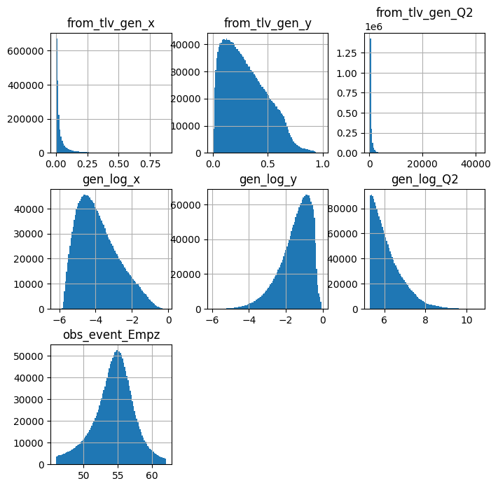
pandas_df.hist( figsize=(8,8), bins=100, column=['from_tlv_gen_x','from_tlv_gen_y','from_tlv_gen_Q2',
                        'gen_log_x','gen_log_y','gen_log_Q2','obs_event_Empz',
                        ])
plt.show()

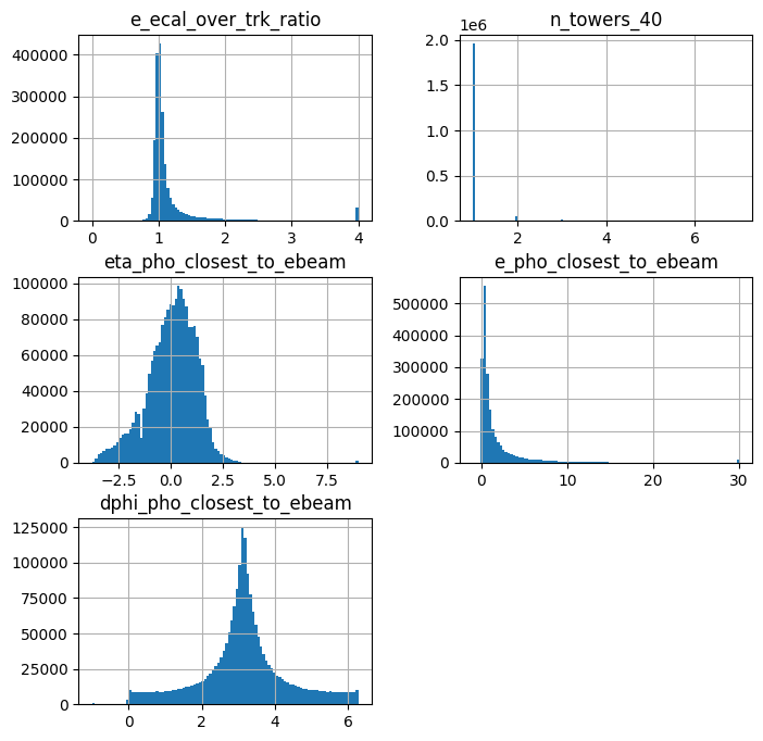
pandas_df.hist( figsize=(8,8), bins=100, column=[
                        'e_ecal_over_trk_ratio','n_towers_40',
                        'eta_pho_closest_to_ebeam','e_pho_closest_to_ebeam', 'dphi_pho_closest_to_ebeam'])

plt.show()

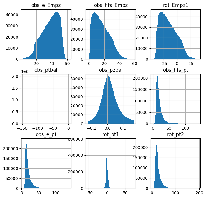
pandas_df.hist( figsize=(8,8), bins=100, column=[
    'obs_e_Empz','obs_hfs_Empz',
    'rot_Empz1',
#    'rot_Empz2',
    'obs_ptbal','obs_pzbal',
    'obs_hfs_pt','obs_e_pt',
    'rot_pt1','rot_pt2'] )

plt.show()

Set up machine learning#

import tensorflow as tf
from tensorflow.keras.layers import Input, Dense, Dropout
from tensorflow.keras.models import Model, Sequential
from sklearn.model_selection import train_test_split
from sklearn.preprocessing import StandardScaler

from pickle import dump

from tensorflow.keras.callbacks import EarlyStopping
earlystopping = EarlyStopping(patience=20,
               verbose=True,
               restore_best_weights=True)

import os

print(tf.config.list_physical_devices())

if has_gpu :
    os.environ['CUDA_VISIBLE_DEVICES']="0"
    physical_devices = tf.config.list_physical_devices('GPU')
    tf.config.experimental.set_memory_growth(physical_devices[0], True)


#####physical_devices = tf.config.list_physical_devices('CPU')

[PhysicalDevice(name='/physical_device:CPU:0', device_type='CPU'), PhysicalDevice(name='/physical_device:GPU:0', device_type='GPU')]

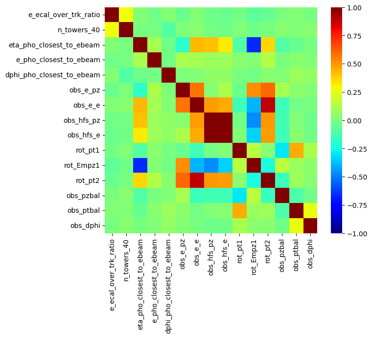
# Let's select the features that are used in the paper

sel_list =  ('e_ecal_over_trk_ratio','n_towers_40','eta_pho_closest_to_ebeam','e_pho_closest_to_ebeam','dphi_pho_closest_to_ebeam','obs_e_pz','obs_e_e','obs_hfs_pz','obs_hfs_e', 'rot_pt1', 'rot_Empz1', 'rot_pt2', 'obs_pzbal', 'obs_ptbal', 'obs_dphi')
sel_list = list(sel_list)

target_list = ('gen_log_x','gen_log_Q2','gen_log_y')
target_list = list(target_list)

sel_X = pandas_df[sel_list]
target_y = pandas_df[target_list]

sub_df = sel_X[: 1000]
corr_matrix = sub_df.corr()

plt.figure(figsize=(7, 6))

sns.heatmap(corr_matrix, cmap='jet', vmin=-1, vmax=1,
            annot=False, fmt='.2f', xticklabels=sub_df.columns, yticklabels=sub_df.columns)
plt.show()

X = sel_X.values

Y_r = target_y.values

GY = pandas_df['from_tlv_gen_y'].to_numpy()

scalerX = StandardScaler()
scalerX.fit(X)
X = scalerX.transform(X)

scalerY = StandardScaler()
scalerY.fit(Y_r)
Y_r = scalerY.transform(Y_r)

#-- Save the scaler transformations!  These are essential when reusing the training with a different dataset.

try:
    os.mkdir( '%s-scalers' % training_extname )
except:
    print('\n  Dir %s-scalers already exists\n\n' % training_extname )


print('\n\n Saving the input and learning target scalers:\n')
print('    %s-scalers/input_scaler.pkl' % training_extname )
print('    %s-scalers/target_scaler.pkl' % training_extname )

dump( scalerX, open('%s-scalers/input_scaler.pkl' % training_extname , 'wb'))
dump( scalerY, open('%s-scalers/target_scaler.pkl' % training_extname , 'wb'))

X_train, X_test, Y_r_train, Y_r_test, GY_train, GY_test = train_test_split( X,  Y_r, GY,  test_size=0.5)

  Dir /content/drive/My Drive/projects/DIS-reco/DIS-reco-paper/training_h1_reg_hugs23_v2-scalers already exists

 Saving the input and learning target scalers:

    /content/drive/My Drive/projects/DIS-reco/DIS-reco-paper/training_h1_reg_hugs23_v2-scalers/input_scaler.pkl
    /content/drive/My Drive/projects/DIS-reco/DIS-reco-paper/training_h1_reg_hugs23_v2-scalers/target_scaler.pkl

print(type(X),np.shape(X))

<class 'numpy.ndarray'> (2027827, 15)

print(np.shape(X_train),np.shape(Y_r_train))
print(np.shape(X_test),np.shape(Y_r_test))
print("GY_train shape: ",np.shape(GY_train))
print("GY_test shape: ",np.shape(GY_test))

(1013913, 15) (1013913, 3)
(1013914, 15) (1013914, 3)
GY_train shape:  (1013913,)
GY_test shape:  (1013914,)

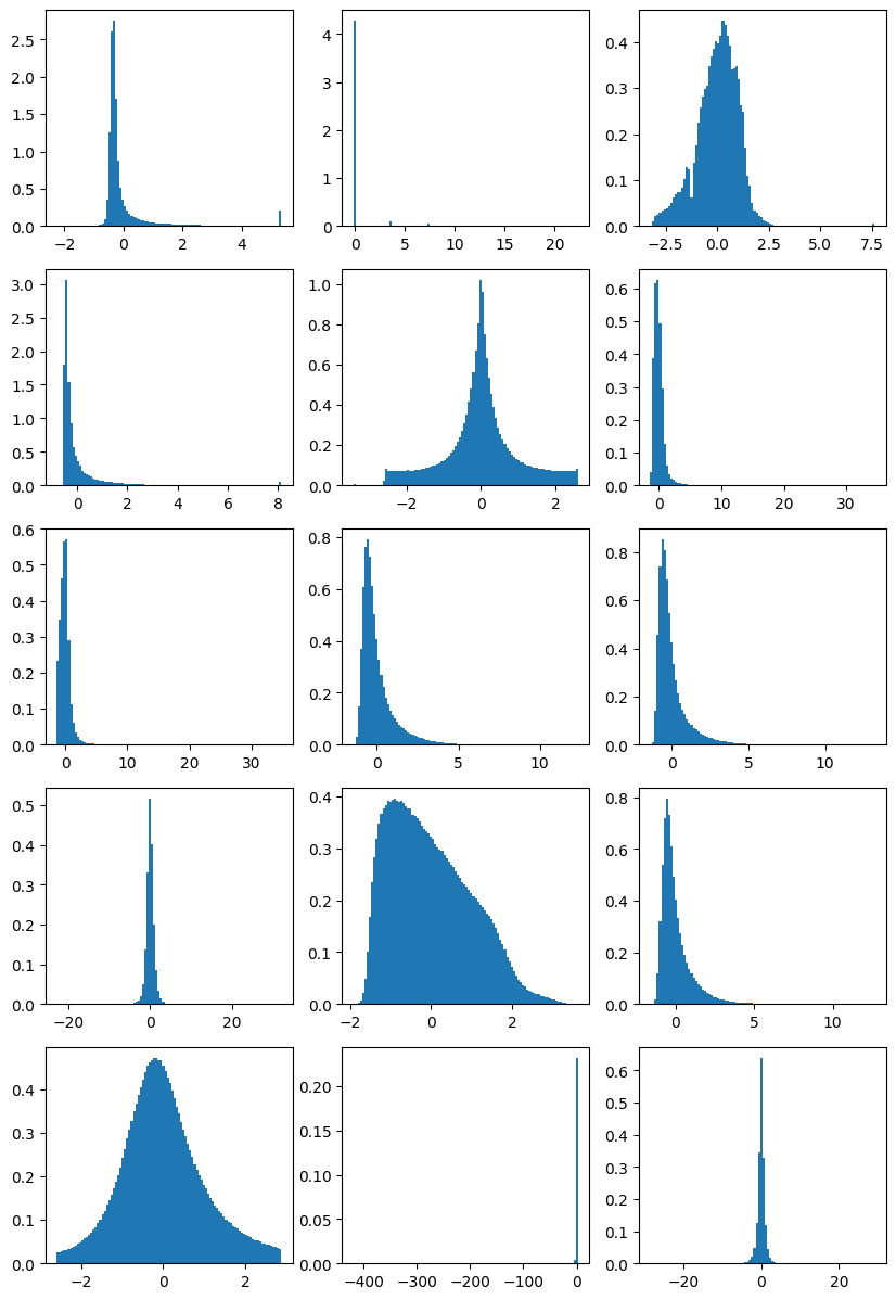
fig, ax = plt.subplots(5, 3, figsize=(10, 15))

for i in range(5):
    for j in range(3):
        idx = i * 3 + j
        if idx < X.shape[1]:  # check if we're still within the number of columns in X
            ax[i][j].hist(X[:, idx], density=True, bins=100)
        else:
            ax[i][j].axis('off')  # turn off remaining axes

plt.show()

Set up the regression network#

model_r = Sequential()

#-- initial layer
model_r.add(Dense(64, input_dim=15, activation='relu'))
model_r.add(Dropout(dropout_setval))

#-- middle part
model_r.add(Dense(128, activation='selu'))
model_r.add(Dropout(dropout_setval))
model_r.add(Dense(512, activation='selu'))
model_r.add(Dropout(dropout_setval))
model_r.add(Dense(1024, activation='selu'))
model_r.add(Dropout(dropout_setval))
model_r.add(Dense(512, activation='selu'))
model_r.add(Dropout(dropout_setval))
model_r.add(Dense(128, activation='selu'))
model_r.add(Dropout(dropout_setval))

#-- final layers
model_r.add(Dense(64, activation='selu'))
model_r.add(Dense(3, activation='linear'))

opt_r = tf.keras.optimizers.Adam( learning_rate=learning_rate_setval_reg, amsgrad=amsgrad_setval )
myloss_r = tf.keras.losses.Huber( delta=delta_setval )

#model_r.compile(loss=myloss_r, optimizer=opt_r, metrics=['mean_absolute_error'])
model_r.compile(loss=myloss_r, optimizer=opt_r)

model_r.summary()

Model: "sequential"
_________________________________________________________________
 Layer (type)                Output Shape              Param #   
=================================================================
 dense (Dense)               (None, 64)                1024      
                                                                 
 dropout (Dropout)           (None, 64)                0         
                                                                 
 dense_1 (Dense)             (None, 128)               8320      
                                                                 
 dropout_1 (Dropout)         (None, 128)               0         
                                                                 
 dense_2 (Dense)             (None, 512)               66048     
                                                                 
 dropout_2 (Dropout)         (None, 512)               0         
                                                                 
 dense_3 (Dense)             (None, 1024)              525312    
                                                                 
 dropout_3 (Dropout)         (None, 1024)              0         
                                                                 
 dense_4 (Dense)             (None, 512)               524800    
                                                                 
 dropout_4 (Dropout)         (None, 512)               0         
                                                                 
 dense_5 (Dense)             (None, 128)               65664     
                                                                 
 dropout_5 (Dropout)         (None, 128)               0         
                                                                 
 dense_6 (Dense)             (None, 64)                8256      
                                                                 
 dense_7 (Dense)             (None, 3)                 195       
                                                                 
=================================================================
Total params: 1,199,619
Trainable params: 1,199,619
Non-trainable params: 0
_________________________________________________________________

%%time

hist_r = model_r.fit(
    X_train, Y_r_train,
    epochs=max_epochs, batch_size=batch_size_setval, verbose=1,
    validation_data=(X_test,Y_r_test),
    callbacks=[earlystopping] )

Epoch 1/50
991/991 [==============================] - 19s 11ms/step - loss: 0.0018 - val_loss: 0.0012
Epoch 2/50
991/991 [==============================] - 8s 8ms/step - loss: 0.0011 - val_loss: 0.0010
Epoch 3/50
991/991 [==============================] - 9s 9ms/step - loss: 9.6870e-04 - val_loss: 9.3596e-04
Epoch 4/50
991/991 [==============================] - 8s 8ms/step - loss: 8.9657e-04 - val_loss: 8.6993e-04
Epoch 5/50
991/991 [==============================] - 7s 7ms/step - loss: 8.4757e-04 - val_loss: 8.3529e-04
Epoch 6/50
991/991 [==============================] - 9s 9ms/step - loss: 8.1183e-04 - val_loss: 8.0680e-04
Epoch 7/50
991/991 [==============================] - 9s 9ms/step - loss: 7.8547e-04 - val_loss: 7.9091e-04
Epoch 8/50
991/991 [==============================] - 8s 8ms/step - loss: 7.6325e-04 - val_loss: 7.5647e-04
Epoch 9/50
991/991 [==============================] - 9s 9ms/step - loss: 7.4459e-04 - val_loss: 7.4042e-04
Epoch 10/50
991/991 [==============================] - 8s 8ms/step - loss: 7.3022e-04 - val_loss: 7.2414e-04
Epoch 11/50
991/991 [==============================] - 9s 9ms/step - loss: 7.1590e-04 - val_loss: 7.1354e-04
Epoch 12/50
991/991 [==============================] - 9s 9ms/step - loss: 7.0551e-04 - val_loss: 7.0036e-04
Epoch 13/50
991/991 [==============================] - 8s 8ms/step - loss: 6.9453e-04 - val_loss: 7.0031e-04
Epoch 14/50
991/991 [==============================] - 9s 9ms/step - loss: 6.8590e-04 - val_loss: 6.9650e-04
Epoch 15/50
991/991 [==============================] - 8s 8ms/step - loss: 6.7717e-04 - val_loss: 6.8033e-04
Epoch 16/50
991/991 [==============================] - 9s 9ms/step - loss: 6.7033e-04 - val_loss: 6.8782e-04
Epoch 17/50
991/991 [==============================] - 9s 9ms/step - loss: 6.6388e-04 - val_loss: 6.7123e-04
Epoch 18/50
991/991 [==============================] - 8s 8ms/step - loss: 6.5735e-04 - val_loss: 6.6752e-04
Epoch 19/50
991/991 [==============================] - 10s 10ms/step - loss: 6.5187e-04 - val_loss: 6.8402e-04
Epoch 20/50
991/991 [==============================] - 10s 11ms/step - loss: 6.4631e-04 - val_loss: 6.5324e-04
Epoch 21/50
991/991 [==============================] - 8s 8ms/step - loss: 6.4133e-04 - val_loss: 6.5073e-04
Epoch 22/50
991/991 [==============================] - 9s 9ms/step - loss: 6.3720e-04 - val_loss: 6.3756e-04
Epoch 23/50
991/991 [==============================] - 8s 8ms/step - loss: 6.3223e-04 - val_loss: 6.4863e-04
Epoch 24/50
991/991 [==============================] - 9s 9ms/step - loss: 6.2849e-04 - val_loss: 6.3588e-04
Epoch 25/50
991/991 [==============================] - 10s 10ms/step - loss: 6.2463e-04 - val_loss: 6.3600e-04
Epoch 26/50
991/991 [==============================] - 8s 8ms/step - loss: 6.2054e-04 - val_loss: 6.3251e-04
Epoch 27/50
991/991 [==============================] - 9s 9ms/step - loss: 6.1795e-04 - val_loss: 6.5578e-04
Epoch 28/50
991/991 [==============================] - 8s 8ms/step - loss: 6.1481e-04 - val_loss: 6.3111e-04
Epoch 29/50
991/991 [==============================] - 8s 8ms/step - loss: 6.1129e-04 - val_loss: 6.1475e-04
Epoch 30/50
991/991 [==============================] - 11s 11ms/step - loss: 6.0822e-04 - val_loss: 6.1605e-04
Epoch 31/50
991/991 [==============================] - 9s 9ms/step - loss: 6.0588e-04 - val_loss: 6.2219e-04
Epoch 32/50
991/991 [==============================] - 8s 8ms/step - loss: 6.0301e-04 - val_loss: 6.1395e-04
Epoch 33/50
991/991 [==============================] - 11s 11ms/step - loss: 6.0020e-04 - val_loss: 6.0387e-04
Epoch 34/50
991/991 [==============================] - 8s 8ms/step - loss: 5.9814e-04 - val_loss: 6.0871e-04
Epoch 35/50
991/991 [==============================] - 8s 8ms/step - loss: 5.9567e-04 - val_loss: 6.0209e-04
Epoch 36/50
991/991 [==============================] - 8s 8ms/step - loss: 5.9355e-04 - val_loss: 5.9776e-04
Epoch 37/50
991/991 [==============================] - 8s 8ms/step - loss: 5.9091e-04 - val_loss: 5.9876e-04
Epoch 38/50
991/991 [==============================] - 8s 8ms/step - loss: 5.9029e-04 - val_loss: 5.9862e-04
Epoch 39/50
991/991 [==============================] - 7s 7ms/step - loss: 5.8710e-04 - val_loss: 5.8963e-04
Epoch 40/50
991/991 [==============================] - 8s 9ms/step - loss: 5.8547e-04 - val_loss: 6.0413e-04
Epoch 41/50
991/991 [==============================] - 8s 8ms/step - loss: 5.8332e-04 - val_loss: 6.0851e-04
Epoch 42/50
991/991 [==============================] - 8s 8ms/step - loss: 5.8195e-04 - val_loss: 5.9649e-04
Epoch 43/50
991/991 [==============================] - 9s 9ms/step - loss: 5.8016e-04 - val_loss: 5.9112e-04
Epoch 44/50
991/991 [==============================] - 7s 7ms/step - loss: 5.7821e-04 - val_loss: 5.8393e-04
Epoch 45/50
991/991 [==============================] - 9s 9ms/step - loss: 5.7687e-04 - val_loss: 5.7991e-04
Epoch 46/50
991/991 [==============================] - 10s 10ms/step - loss: 5.7440e-04 - val_loss: 5.8244e-04
Epoch 47/50
991/991 [==============================] - 8s 8ms/step - loss: 5.7386e-04 - val_loss: 6.0049e-04
Epoch 48/50
991/991 [==============================] - 9s 9ms/step - loss: 5.7166e-04 - val_loss: 5.7298e-04
Epoch 49/50
991/991 [==============================] - 7s 7ms/step - loss: 5.7087e-04 - val_loss: 5.7640e-04
Epoch 50/50
991/991 [==============================] - 9s 9ms/step - loss: 5.6885e-04 - val_loss: 5.7290e-04
CPU times: user 6min 42s, sys: 22.3 s, total: 7min 4s
Wall time: 7min 23s

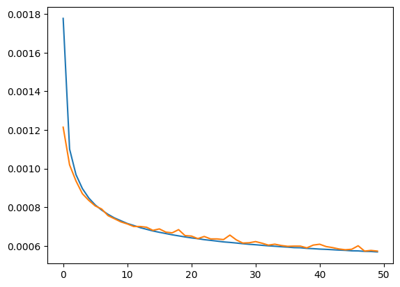
plt.plot(hist_r.history['loss'])
plt.plot(hist_r.history['val_loss'])

[<matplotlib.lines.Line2D at 0x7fca4a75e170>]

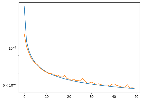
plt.plot(hist_r.history['loss'])
plt.plot(hist_r.history['val_loss'])
plt.yscale('log')

filepath_model = training_extname + "_regression"

tf.keras.models.save_model(model_r,filepath_model)

mypreds_r = model_r.predict(X_test,batch_size=1000)

1014/1014 [==============================] - 2s 2ms/step

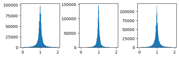
fig,ax = plt.subplots(1,3,figsize=(7,2))
ax[0].hist(mypreds_r[:,0]/Y_r_test[:,0],bins=100, range=[0,2] )
ax[1].hist(mypreds_r[:,1]/Y_r_test[:,1],bins=100, range=[0,2] )
ax[2].hist(mypreds_r[:,2]/Y_r_test[:,2],bins=100, range=[0,2] )
plt.subplots_adjust(wspace=0.5)
plt.show()

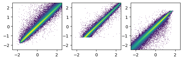
fig,ax = plt.subplots(1,3,figsize=(7,2))
ax[0].hist2d(mypreds_r[:,0],Y_r_test[:,0],bins=200, norm=mpl.colors.LogNorm(), range=([-2.5,2.5],[-2.5,2.5]))
ax[1].hist2d(mypreds_r[:,1],Y_r_test[:,1],bins=200, norm=mpl.colors.LogNorm(), range=([-2.5,2.5],[-2.5,2.5]))
ax[2].hist2d(mypreds_r[:,2],Y_r_test[:,2],bins=200, norm=mpl.colors.LogNorm(), range=([-2.5,2.5],[-2.5,2.5]))
plt.show()

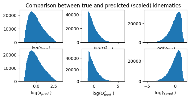
fig,ax = plt.subplots(2,3,figsize=(7,3), sharex='col')

# define titles and x-labels
true_labels = ['log(x$_{true})$', 'log(Q$^2_{true})$', 'log(y$_{true})$']
pred_labels = ['log(x$_{pred.})$', 'log(Q$^2_{pred.})$', 'log(y$_{pred.})$']

ax[0][1].set_title("Comparison between true and predicted (scaled) kinematics") # title for the first row

for i in range(3):
    ax[0][i].hist(Y_r_test[:,i], bins=100)
    ax[0][i].set_xlabel(true_labels[i]) # x-label for the upper plots

    ax[1][i].hist(mypreds_r[:,i], bins=100)
    ax[1][i].set_xlabel(pred_labels[i]) # x-label for the lower plots

plt.subplots_adjust(wspace=0.45)
plt.show()

# Inverse transform to their unscaled values (i.e., before standard scaling)

inv_trans_Y = scalerY.inverse_transform(Y_r_test)
inv_trans_pred = scalerY.inverse_transform(mypreds_r)
true_vals = np.exp( inv_trans_Y)
pred_vals = np.exp( inv_trans_pred)

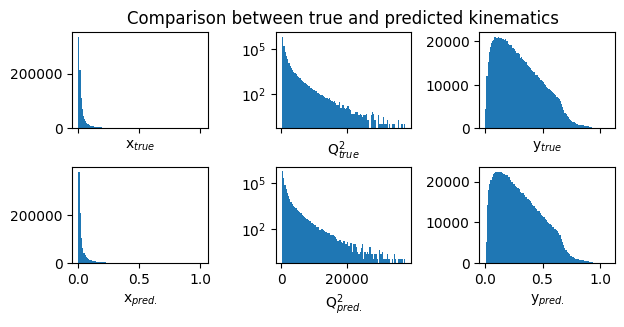
fig,ax = plt.subplots(2,3,figsize=(7,3), sharex='col')

# define titles and x-labels
true_labels = ['x$_{true}$', 'Q$^2_{true}$', 'y$_{true}$']
pred_labels = ['x$_{pred.}$', 'Q$^2_{pred.}$', 'y$_{pred.}$']

ax[0][1].set_title("Comparison between true and predicted kinematics") # title for the first row

for i in range(3):
    ax[0][i].hist(true_vals[:,i], bins=100)
    ax[0][i].set_xlabel(true_labels[i]) # x-label for the upper plots

    ax[1][i].hist(pred_vals[:,i], bins=100)
    ax[1][i].set_xlabel(pred_labels[i]) # x-label for the lower plots

ax[0][1].set_yscale('log')
ax[1][1].set_yscale('log')

plt.subplots_adjust(hspace=0.4)
plt.subplots_adjust(wspace=0.5)
plt.show()

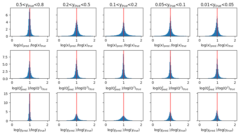
Plots of Ratio(pred/true) for target variables : transformed log(x), log(y), and log(Q2)#

fig, ax = plt.subplots(3,5, figsize=(12,6), sharey='row')

titles = ['log(x)$_{pred.}$/log(x)$_{true}$', 'log(Q$^2_{pred.}$)/log(Q$^2$)$_{true}$', 'log(y$_{pred.}$)/log(y$_{true}$)']
y_ranges = [
    (0.5, 0.8),
    (0.2, 0.5),
    (0.1, 0.2),
    (0.05, 0.1),
    (0.01, 0.05)
]

for i in range(3):
    for j in range(5):
        y_min, y_max = y_ranges[j]
        mask = (GY_test > y_min)*(GY_test < y_max)
        ax[i][j].hist(mypreds_r[:,i][mask]/Y_r_test[mask][:,i],
                      density=True,bins=100,range=(0,2))
        ax[i][j].axvline(1.0, color='red', lw=2, alpha=0.6)
        ax[i][j].set_xlabel(titles[i])  # set column x-label

        if i == 0:
            ax[i][j].set_title(f'{y_min}<y$_{{true}}$<{y_max}')

plt.subplots_adjust(hspace=0.5)
plt.show()

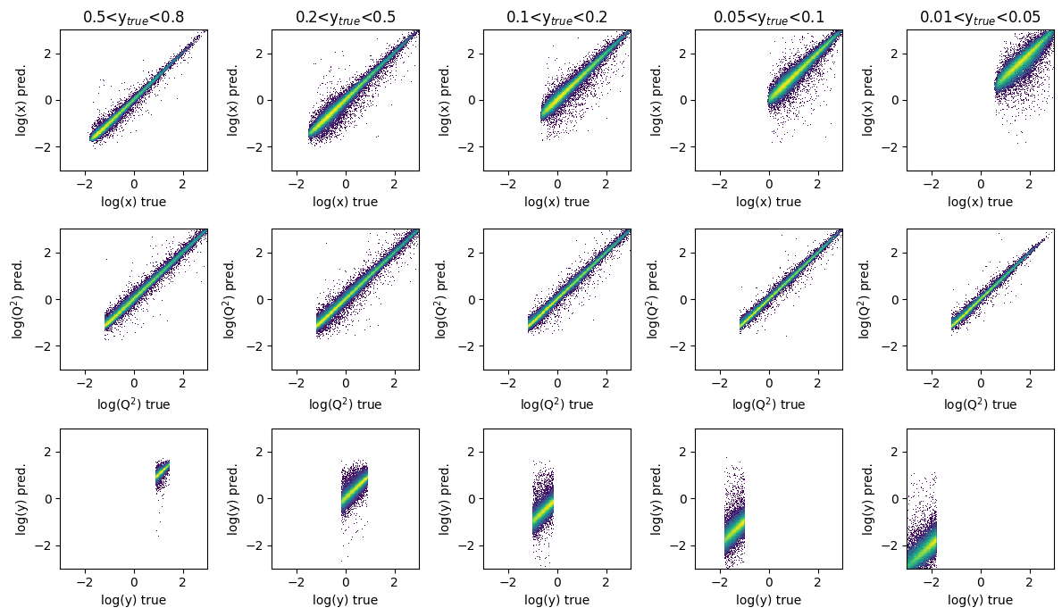
fig, ax = plt.subplots(3, 5, figsize=(12, 7))

titles = ['log(x)', 'log(Q$^2$)', 'log(y)']
y_ranges = [
    (0.5, 0.8),
    (0.2, 0.5),
    (0.1, 0.2),
    (0.05, 0.1),
    (0.01, 0.05)
]

for i in range(3):
    for j in range(5):
        y_min, y_max = y_ranges[j]
        mask = (GY_test > y_min)*(GY_test < y_max)
        ax[i][j].hist2d(Y_r_test[mask][:,i],
                        mypreds_r[:,i][mask],
                        density=True,bins=200,range=([-3,3],[-3,3]),
                        norm=mpl.colors.LogNorm())

        if i == 0:
            ax[i][j].set_title(f'{y_min}<y$_{{true}}$<{y_max}')

        ax[i][j].set_ylabel(titles[i] + ' pred.')
        ax[i][j].set_xlabel(titles[i] + ' true')

plt.tight_layout()
plt.show()

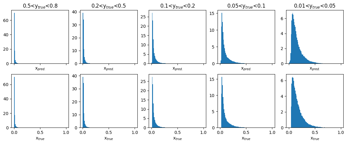
Plots of predicted and true physics variable : x#

fig,ax = plt.subplots(2,5,figsize=(14,5),sharex='col')

y_ranges = [(0.5, 0.8),(0.2, 0.5),(0.1, 0.2),(0.05, 0.1),(0.01, 0.05)]

for i in range(2):
    for j in range(5):
        y_min, y_max = y_ranges[j]
        mask = (GY_test > y_min)*(GY_test < y_max)
        if i == 0:
            ax[i][j].hist(pred_vals[:,0][mask],density=True,bins=100,range=(0,1))
            ax[i][j].set_title(f'{y_min}<y$_{{true}}$<{y_max}')
            ax[i][j].set_xlabel('x$_{pred.}$')
        else:
            ax[i][j].hist(true_vals[:,0][mask],density=True,bins=100,range=(0,1))
            ax[i][j].set_xlabel('x$_{true}$')

plt.show()

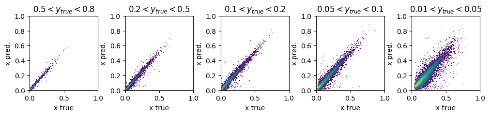
fig, ax = plt.subplots(1,5, figsize=(12,2))

y_ranges = [(0.5, 0.8), (0.2, 0.5), (0.1, 0.2), (0.05, 0.1), (0.01, 0.05)]
titles = ['$0.5<y_{true}<0.8$', '$0.2<y_{true}<0.5$', '$0.1<y_{true}<0.2$', '$0.05<y_{true}<0.1$', '$0.01<y_{true}<0.05$']

for i in range(5):
    y_min, y_max = y_ranges[i]
    mask = (GY_test > y_min) * (GY_test < y_max)
    ax[i].hist2d(true_vals[:,0][mask], pred_vals[:,0][mask],
                 density=True, bins=200, range=([0,1],[0,1]), norm=mpl.colors.LogNorm())
    ax[i].set_title(titles[i])
    ax[i].set_xlabel('x true')
    ax[i].set_ylabel('x pred.')


plt.subplots_adjust(wspace=0.4)

plt.show()

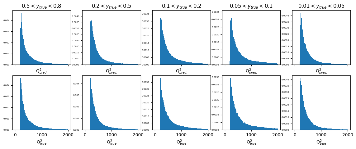
Plots of predicted and true physics variable : Q2#

fig, ax = plt.subplots(2, 5, figsize=(14, 5), sharex='col')

y_ranges = [(0.5, 0.8), (0.2, 0.5), (0.1, 0.2), (0.05, 0.1), (0.01, 0.05)]
xmax = 2000
titles = ['$0.5<y_{true}<0.8$', '$0.2<y_{true}<0.5$', '$0.1<y_{true}<0.2$', '$0.05<y_{true}<0.1$', '$0.01<y_{true}<0.05$']
x_labels = ['Q$^{2}_{pred.}$', 'Q$^{2}_{true}$']

for i in range(2):
    for j in range(5):
        y_min, y_max = y_ranges[j]
        mask = (GY_test > y_min)*(GY_test < y_max)
        ax[i][j].hist(pred_vals[:,1][mask] if i == 0 else true_vals[:,1][mask],
                      density=True, bins=100, range=(0, xmax))
        if i==0:
          ax[i][j].set_title(titles[j])
        ax[i][j].set_xlabel(x_labels[i])
        ax[i][j].tick_params(axis='y', labelsize=5)  # adjust the fontsize of y-axis

plt.show()

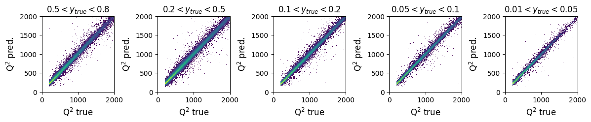
fig, ax = plt.subplots(1, 5, figsize=(14, 2))
axis_max = 2000

y_ranges = [(0.5, 0.8), (0.2, 0.5), (0.1, 0.2), (0.05, 0.1), (0.01, 0.05)]
titles = ['$0.5 < y_{true} < 0.8$', '$0.2 < y_{true} < 0.5$', '$0.1 < y_{true} < 0.2$', '$0.05 < y_{true} < 0.1$', '$0.01 < y_{true} < 0.05$']
x_label = 'Q$^{2}$ true'
y_label = 'Q$^{2}$ pred.'

for i in range(5):
    y_min, y_max = y_ranges[i]
    mask = (GY_test > y_min) * (GY_test < y_max)
    ax[i].hist2d(true_vals[:, 1][mask], pred_vals[:, 1][mask],
                 density=True, bins=200, range=([0, axis_max], [0, axis_max]), norm=mpl.colors.LogNorm())
    ax[i].set_title(titles[i])
    ax[i].set_ylabel('Q$^{2}$ pred.')
    ax[i].set_xlabel(x_label)
    ax[i].set_xlabel(x_label, fontsize=12)
    ax[i].set_ylabel(y_label, fontsize=12)

plt.subplots_adjust(wspace=0.6)
plt.show()

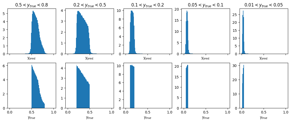
Plots of predicted and true physics variable : y#

fig, ax = plt.subplots(2, 5, figsize=(14, 5), sharex='col')
xmax = 1

y_ranges = [(0.5, 0.8), (0.2, 0.5), (0.1, 0.2), (0.05, 0.1), (0.01, 0.05)]
titles = ['$0.5 < y_{true} < 0.8$', '$0.2 < y_{true} < 0.5$', '$0.1 < y_{true} < 0.2$', '$0.05 < y_{true} < 0.1$', '$0.01 < y_{true} < 0.05$']
x_label = ['y$_{pred.}$','y$_{true}$']

for i in range(5):
    y_min, y_max = y_ranges[i]
    mask = (GY_test > y_min) * (GY_test < y_max)
    ax[0][i].hist(pred_vals[:, 2][mask], density=True, bins=100, range=(0, xmax))
    ax[1][i].hist(true_vals[:, 2][mask], density=True, bins=100, range=(0, xmax))
    ax[0][i].set_title(titles[i])
    ax[0][i].set_xlabel(x_label[0])
    ax[1][i].set_xlabel(x_label[1])

plt.show()

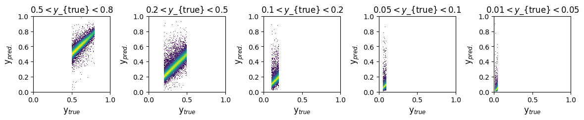
fig, ax = plt.subplots(1, 5, figsize=(14, 2))
axis_max = 1

y_ranges = [(0.5, 0.8), (0.2, 0.5), (0.1, 0.2), (0.05, 0.1), (0.01, 0.05)]
titles = ['$0.5 < y$_{true}$ < 0.8$', '$0.2 < y$_{true}$ < 0.5$', '$0.1 < y$_{true}$ < 0.2$', '$0.05 < y$_{true}$ < 0.1$', '$0.01 < y$_{true}$ < 0.05$']
x_label = 'y$_{true}$'
y_label = 'y$_{pred.}$'

for i in range(5):
    y_min, y_max = y_ranges[i]
    mask = (GY_test > y_min) * (GY_test < y_max)
    ax[i].hist2d(true_vals[:, 2][mask], pred_vals[:, 2][mask], density=True, bins=200, range=([0, axis_max], [0, axis_max]), norm=mpl.colors.LogNorm())
    ax[i].set_title(titles[i])
    ax[i].set_xlabel(x_label)
    ax[i].set_ylabel(y_label)
    ax[i].set_xlabel(x_label, fontsize=12)
    ax[i].set_ylabel(y_label, fontsize=12)

plt.subplots_adjust(wspace=0.5)
plt.show()

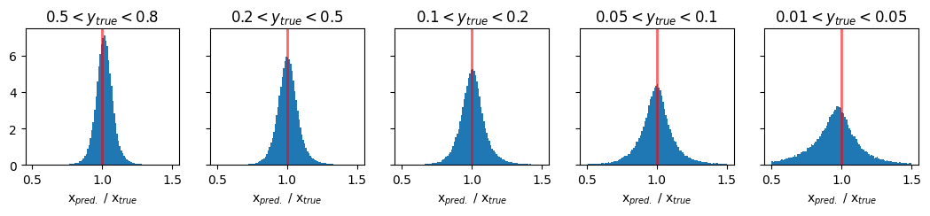
Plots of pred/true of physics variable x#

fig, ax = plt.subplots(1, 5, figsize=(13, 2), sharey='row')
xmin = 0.5
xmax = 1.5
y_ranges = [(0.5, 0.8), (0.2, 0.5), (0.1, 0.2), (0.05, 0.1), (0.01, 0.05)]
titles = ['$0.5 < y_{true} < 0.8$', '$0.2 < y_{true} < 0.5$', '$0.1 < y_{true} < 0.2$', '$0.05 < y_{true} < 0.1$', '$0.01 < y_{true} < 0.05$']

for i in range(5):
    y_min, y_max = y_ranges[i]
    mask = (GY_test > y_min) * (GY_test < y_max)
    ax[i].hist(pred_vals[:, 0][mask] / true_vals[:, 0][mask], density=True, bins=100, range=(xmin, xmax))
    ax[i].set_title(titles[i])
    ax[i].axvline(1.0, color='red', lw=2, alpha=0.6)
    ax[i].set_xlabel('x$_{pred.}$ / x$_{true}$')

plt.show()

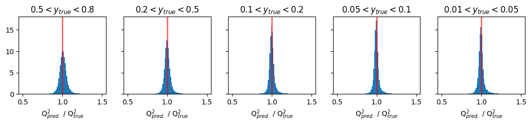
Plots of pred/true of physics variable Q2#

fig, ax = plt.subplots(1, 5, figsize=(13, 2), sharey='row')
xmin = 0.5
xmax = 1.5
y_ranges = [(0.5, 0.8), (0.2, 0.5), (0.1, 0.2), (0.05, 0.1), (0.01, 0.05)]
titles = ['$0.5 < y_{true} < 0.8$', '$0.2 < y_{true} < 0.5$', '$0.1 < y_{true} < 0.2$', '$0.05 < y_{true} < 0.1$', '$0.01 < y_{true} < 0.05$']

for i in range(5):
    y_min, y_max = y_ranges[i]
    mask = (GY_test > y_min) * (GY_test < y_max)
    ax[i].hist(pred_vals[:, 1][mask] / true_vals[:, 1][mask], density=True, bins=100, range=(xmin, xmax))
    ax[i].set_title(titles[i])
    ax[i].axvline(1.0, color='red', lw=2, alpha=0.6)
    ax[i].set_xlabel('Q$^{2}_{pred.}$ / Q$^{2}_{true}$')

plt.show()

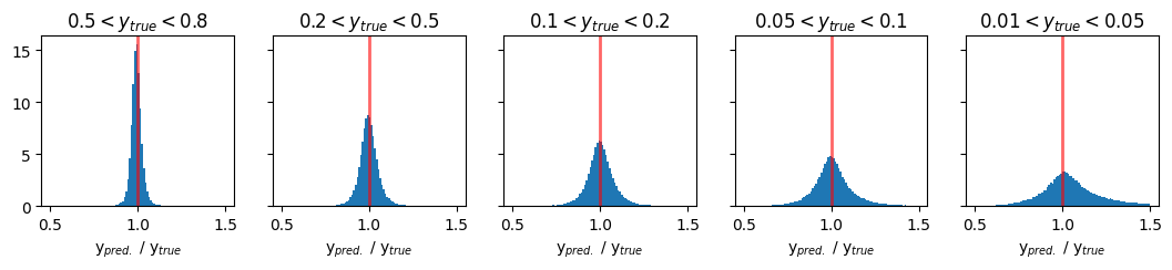
Plots of pred/true of physics variable y#

fig, ax = plt.subplots(1, 5, figsize=(13, 2), sharey='row')
xmin = 0.5
xmax = 1.5
y_ranges = [(0.5, 0.8), (0.2, 0.5), (0.1, 0.2), (0.05, 0.1), (0.01, 0.05)]
titles = ['$0.5 < y_{true} < 0.8$', '$0.2 < y_{true} < 0.5$', '$0.1 < y_{true} < 0.2$', '$0.05 < y_{true} < 0.1$', '$0.01 < y_{true} < 0.05$']

for i in range(5):
    y_min, y_max = y_ranges[i]
    mask = (GY_test > y_min) * (GY_test < y_max)
    ax[i].hist(pred_vals[:, 2][mask] / true_vals[:, 2][mask], density=True, bins=100, range=(xmin, xmax))
    ax[i].set_title(titles[i])
    ax[i].axvline(1.0, color='red', lw=2, alpha=0.6)
    ax[i].set_xlabel('y$_{pred.}$ / y$_{true}$')

plt.show()

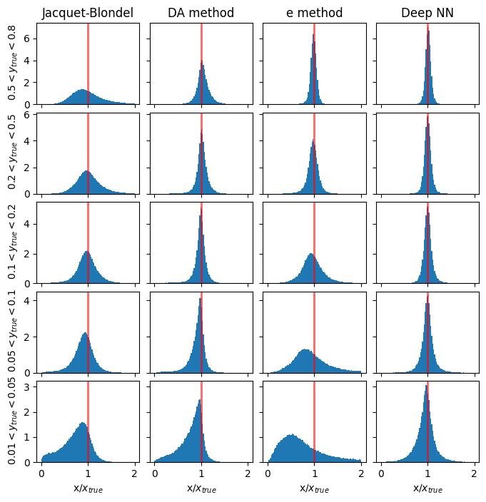
Comparison plots of resolution for methods vs DNN#

Resolution in x#

# y_ranges = [ (0.5, 0.8), (0.2, 0.5), (0.1, 0.2), (0.05, 0.1), (0.01, 0.05)] #---previously defined

mean_xratio = []
rms_xratio = []

def cal_mean_rms(bin_edges,counts, mean_l, rms_l):
  bin_centers = 0.5 * (bin_edges[1:] + bin_edges[:-1])
  mean = np.average(bin_centers, weights=counts)
  rms = np.sqrt(np.average((bin_centers - mean) ** 2, weights=counts))
  mean_l.append(mean)
  rms_l.append(rms)
  return mean_l, rms_l

methods_to_use = [4, 3, 0] # [5, 4, 3, 0]
methods_labels = ['Jacquet-Blondel', 'DA method', 'e method', 'Deep NN'] #'I$\Sigma$ method', 'Jacquet-Blondel', 'DA method', 'e method', 'Deep NN'
xmin = 0.0
xmax = 2.0
y_cut = ['from_tlv_gen_y>0.50 and from_tlv_gen_y<0.80','from_tlv_gen_y>0.20 and from_tlv_gen_y<0.50','from_tlv_gen_y>0.10 and from_tlv_gen_y<0.20','from_tlv_gen_y>0.05 and from_tlv_gen_y<0.10','from_tlv_gen_y>0.01 and from_tlv_gen_y<0.05']

fig, ax = plt.subplots(len(y_cut), len(methods_labels), figsize=(8, 8), sharey='row', sharex=True)


# the standard methods
for i in range(len(methods_to_use)):
    mi = methods_to_use[i]
    for yi in range(len(y_cut)):
        counts, bin_edges, _ = ax[yi][i].hist(pandas_df.query(y_cut[yi])['obs_x[%d]' % mi] / pandas_df.query(y_cut[yi])['from_tlv_gen_x'],
                       density=True, bins=100, range=(xmin, xmax))
        if(yi==0):
          ax[yi][i].set_title(methods_labels[i])

        mean_xratio, rms_xratio= cal_mean_rms(bin_edges,counts, mean_xratio, rms_xratio)



# the DNN method
for yi in range(len(y_cut)):
    counts, bin_edges, _ = ax[yi][len(methods_to_use)].hist(pred_vals[:, 0][(GY_test > y_ranges[yi][0]) * (GY_test < y_ranges[yi][1])] / true_vals[:, 0][(GY_test > y_ranges[yi][0]) * (GY_test < y_ranges[yi][1])],
                   density=True, bins=100, range=(xmin, xmax))
    ax[0][len(methods_to_use)].set_title('Deep NN')

    mean_xratio, rms_xratio= cal_mean_rms(bin_edges,counts, mean_xratio, rms_xratio)


for yi, y_range in enumerate(y_ranges):
    ax[yi][0].set_ylabel(f' ${y_range[0]} < y_{{true}} < {y_range[1]}$')

if(len(y_cut)>0):
  for i in range(len(methods_to_use)+1):
      ax[len(y_cut)-1][i].set_xlabel('x/$x_{true}$')

for i in range(len(y_cut)):
    for j in range(len(methods_to_use)+1): # +1 to include DNN
        ax[i][j].axvline(1.0, color='red', lw=2, alpha=0.6)


plt.subplots_adjust(wspace=0.1, hspace=0.1)
plt.show()

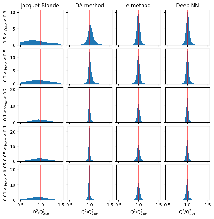
Resolution in Q2#

# y_ranges = [ (0.5, 0.8), (0.2, 0.5), (0.1, 0.2), (0.05, 0.1), (0.01, 0.05)] #---previously defined


mean_Q2ratio = []
rms_Q2ratio = []

methods_to_use = [4, 3, 0] # [5, 4, 3, 0]
methods_labels = ['Jacquet-Blondel', 'DA method', 'e method', 'Deep NN'] #'I$\Sigma$ method', 'Jacquet-Blondel', 'DA method', 'e method', 'Deep NN'
xmin = 0.5
xmax = 1.5
y_cut = ['from_tlv_gen_y>0.50 and from_tlv_gen_y<0.80','from_tlv_gen_y>0.20 and from_tlv_gen_y<0.50','from_tlv_gen_y>0.10 and from_tlv_gen_y<0.20','from_tlv_gen_y>0.05 and from_tlv_gen_y<0.10','from_tlv_gen_y>0.01 and from_tlv_gen_y<0.05']

fig, ax = plt.subplots(len(y_cut), len(methods_labels), figsize=(8, 8), sharey='row', sharex=True)


# the standard methods
for i in range(len(methods_to_use)):
    mi = methods_to_use[i]
    for yi in range(len(y_cut)):
        counts, bin_edges, _ = ax[yi][i].hist(pandas_df.query(y_cut[yi])['obs_Q2[%d]' % mi] / pandas_df.query(y_cut[yi])['from_tlv_gen_Q2'],
                       density=True, bins=100, range=(xmin, xmax))
        if(yi==0):
          ax[yi][i].set_title(methods_labels[i])

        mean_Q2ratio, rms_Q2ratio= cal_mean_rms(bin_edges,counts, mean_Q2ratio, rms_Q2ratio)


# the DNN method
for yi in range(len(y_cut)):
    counts, bin_edges, _ =  ax[yi][len(methods_to_use)].hist(pred_vals[:, 1][(GY_test > y_ranges[yi][0]) * (GY_test < y_ranges[yi][1])] / true_vals[:, 1][(GY_test > y_ranges[yi][0]) * (GY_test < y_ranges[yi][1])],
                   density=True, bins=100, range=(xmin, xmax))
    ax[0][len(methods_to_use)].set_title('Deep NN')

    mean_Q2ratio, rms_Q2ratio= cal_mean_rms(bin_edges,counts, mean_Q2ratio, rms_Q2ratio)


for yi, y_range in enumerate(y_ranges):
    ax[yi][0].set_ylabel(f' ${y_range[0]} < y_{{true}} < {y_range[1]}$')

if(len(y_cut)>0):
  for i in range(len(methods_to_use)+1):
      ax[len(y_cut)-1][i].set_xlabel('Q$^2$/Q$^2_{true}$')

for i in range(len(y_cut)):
    for j in range(len(methods_to_use)+1): # +1 to include DNN
        ax[i][j].axvline(1.0, color='red', lw=2, alpha=0.6)


plt.subplots_adjust(wspace=0.1, hspace=0.1)
plt.show()

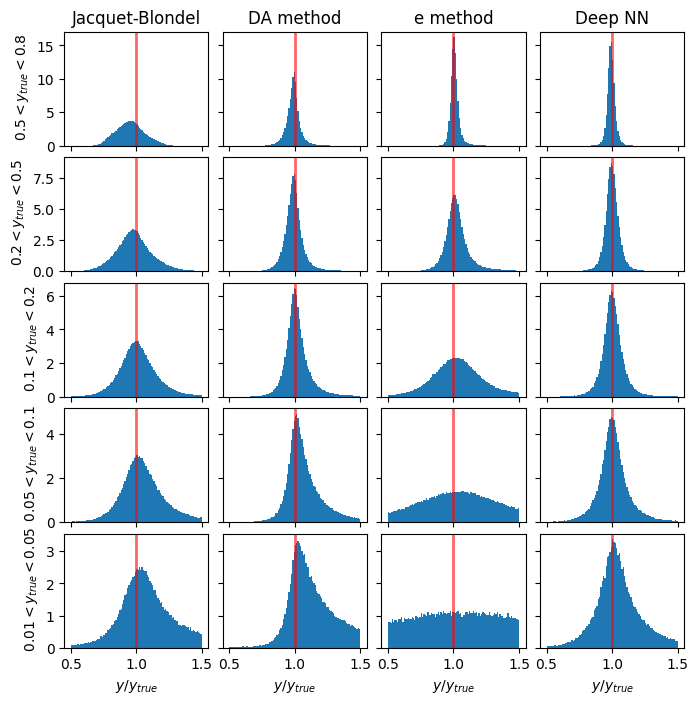
Resolution in y#

# y_ranges = [ (0.5, 0.8), (0.2, 0.5), (0.1, 0.2), (0.05, 0.1), (0.01, 0.05)] #---previously defined

mean_yratio = []
rms_yratio = []

methods_to_use = [4, 3, 0] # [5, 4, 3, 0]
methods_labels = ['Jacquet-Blondel', 'DA method', 'e method', 'Deep NN'] #'I$\Sigma$ method', 'Jacquet-Blondel', 'DA method', 'e method', 'Deep NN'
xmin = 0.5
xmax = 1.5
y_cut = ['from_tlv_gen_y>0.50 and from_tlv_gen_y<0.80','from_tlv_gen_y>0.20 and from_tlv_gen_y<0.50','from_tlv_gen_y>0.10 and from_tlv_gen_y<0.20','from_tlv_gen_y>0.05 and from_tlv_gen_y<0.10','from_tlv_gen_y>0.01 and from_tlv_gen_y<0.05']

fig, ax = plt.subplots(len(y_cut), len(methods_labels), figsize=(8, 8), sharey='row', sharex=True)


# the standard methods
for i in range(len(methods_to_use)):
    mi = methods_to_use[i]
    for yi in range(len(y_cut)):
        counts, bin_edges, _ = ax[yi][i].hist(pandas_df.query(y_cut[yi])['obs_y[%d]' % mi] / pandas_df.query(y_cut[yi])['from_tlv_gen_y'],
                       density=True, bins=100, range=(xmin, xmax))
        if(yi==0):
          ax[yi][i].set_title(methods_labels[i])

        mean_yratio, rms_yratio= cal_mean_rms(bin_edges,counts, mean_yratio, rms_yratio)



# the DNN method
for yi in range(len(y_cut)):
    counts, bin_edges, _ = ax[yi][len(methods_to_use)].hist(pred_vals[:, 2][(GY_test > y_ranges[yi][0]) * (GY_test < y_ranges[yi][1])] / true_vals[:, 2][(GY_test > y_ranges[yi][0]) * (GY_test < y_ranges[yi][1])],
                   density=True, bins=100, range=(xmin, xmax))
    ax[0][len(methods_to_use)].set_title('Deep NN')

    mean_yratio, rms_yratio= cal_mean_rms(bin_edges,counts, mean_yratio, rms_yratio)



for yi, y_range in enumerate(y_ranges):
    ax[yi][0].set_ylabel(f' ${y_range[0]} < y_{{true}} < {y_range[1]}$')

if(len(y_cut)>0):
  for i in range(len(methods_to_use)+1):
      ax[len(y_cut)-1][i].set_xlabel('$y/y_{true}$')

for i in range(len(y_cut)):
    for j in range(len(methods_to_use)+1): # +1 to include DNN
        ax[i][j].axvline(1.0, color='red', lw=2, alpha=0.6)


plt.subplots_adjust(wspace=0.1, hspace=0.1)
plt.show()

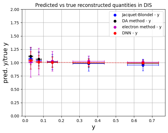
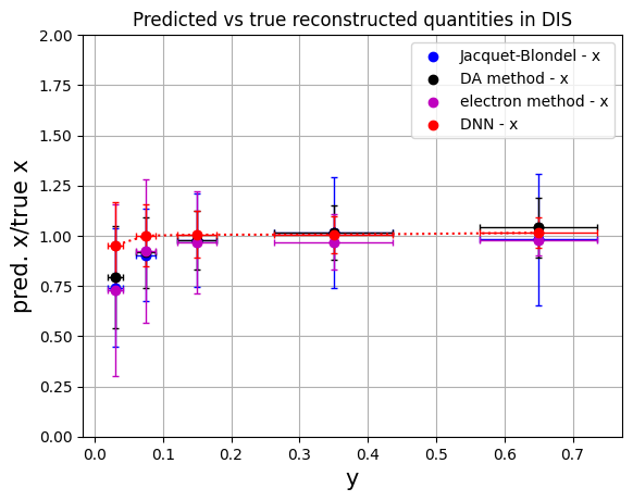
Plotting the results as a function of y#

# convert to numpy arrays for manipulation
# methods: 'Jacquet-Blondel', 'DA method', 'e method', 'Deep NN'

y_ranges = [ (0.5, 0.8), (0.2, 0.5), (0.1, 0.2), (0.05, 0.1), (0.01, 0.05)] #---previously defined

ykin = []
err_ykin = []

for values in y_ranges:
  tmp = 0.5*(values[0]+values[1])
  ykin.append(tmp)
  tmp = abs(values[1]-values[0])
  err_ykin.append(tmp/np.sqrt(12.))

ykin = np.array(ykin)
err_ykin = np.array(err_ykin)


meanx_jb = np.array(mean_xratio[0:5])
errx_jb = np.array(rms_xratio[0:5])

meanx_da = np.array(mean_xratio[5:10])
errx_da = np.array(rms_xratio[5:10])

meanx_e = np.array(mean_xratio[10:15])
errx_e = np.array(rms_xratio[10:15])

meanx_dnn = np.array(mean_xratio[15:20])
errx_dnn = np.array(rms_xratio[15:20])

plt.scatter(ykin, meanx_jb, color='b', label='Jacquet-Blondel - x')
plt.errorbar(ykin, meanx_jb, xerr=err_ykin, yerr=errx_jb, fmt='o', color='b', ecolor='b', elinewidth=1, capsize=2) #label='uncertainty'

plt.scatter(ykin, meanx_da, color='k', label='DA method - x')
plt.errorbar(ykin, meanx_da, xerr=err_ykin, yerr=errx_da, fmt='o', color='k', ecolor='k', elinewidth=1, capsize=2)

plt.scatter(ykin, meanx_e, color='m', label='electron method - x')
plt.errorbar(ykin, meanx_e, xerr=err_ykin, yerr=errx_e, fmt='o', color='m', ecolor='m', elinewidth=1, capsize=2)

plt.scatter(ykin, meanx_dnn, color='r', label='DNN - x')
plt.errorbar(ykin, meanx_dnn, xerr=err_ykin, yerr=errx_dnn, fmt='o', color='r', ecolor='r', elinewidth=1, capsize=2, linestyle=':')


plt.xlabel('y',fontsize=15)
plt.ylabel('pred. x/true x',fontsize=15)
plt.ylim(0.,2.)
plt.title('Predicted vs true reconstructed quantities in DIS')
plt.legend()
plt.grid(True)
plt.show()

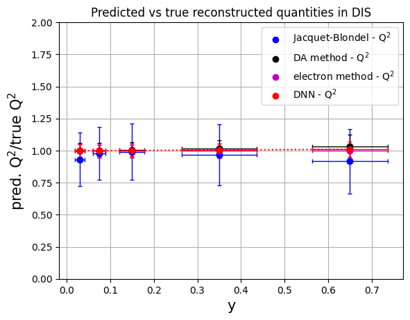
# convert to numpy arrays for manipulation
# methods: 'Jacquet-Blondel', 'DA method', 'e method', 'Deep NN'

y_ranges = [ (0.5, 0.8), (0.2, 0.5), (0.1, 0.2), (0.05, 0.1), (0.01, 0.05)] #---previously defined

meanQ2_jb = np.array(mean_Q2ratio[0:5])
errQ2_jb = np.array(rms_Q2ratio[0:5])

meanQ2_da = np.array(mean_Q2ratio[5:10])
errQ2_da = np.array(rms_Q2ratio[5:10])

meanQ2_e = np.array(mean_Q2ratio[10:15])
errQ2_e = np.array(rms_Q2ratio[10:15])

meanQ2_dnn = np.array(mean_Q2ratio[15:20])
errQ2_dnn = np.array(rms_Q2ratio[15:20])

plt.scatter(ykin, meanQ2_jb, color='b', label='Jacquet-Blondel - Q$^{2}$')
plt.errorbar(ykin, meanQ2_jb, xerr=err_ykin, yerr=errQ2_jb, fmt='o', color='b', ecolor='b', elinewidth=1, capsize=2) #label='uncertainty'

plt.scatter(ykin, meanQ2_da, color='k', label='DA method - Q$^{2}$')
plt.errorbar(ykin, meanQ2_da, xerr=err_ykin, yerr=errQ2_da, fmt='o', color='k', ecolor='k', elinewidth=1, capsize=2)

plt.scatter(ykin, meanQ2_e, color='m', label='electron method - Q$^{2}$')
plt.errorbar(ykin, meanQ2_e, xerr=err_ykin, yerr=errQ2_e, fmt='o', color='m', ecolor='m', elinewidth=1, capsize=2)

plt.scatter(ykin, meanQ2_dnn, color='r', label='DNN - Q$^{2}$')
plt.errorbar(ykin, meanQ2_dnn, xerr=err_ykin, yerr=errQ2_dnn, fmt='o', color='r', ecolor='r', elinewidth=1, capsize=2, linestyle=':')


plt.xlabel('y',fontsize=15)
plt.ylabel('pred. Q$^{2}$/true Q$^{2}$',fontsize=15)
plt.ylim(0.,2.)
plt.title('Predicted vs true reconstructed quantities in DIS')
plt.legend()
plt.grid(True)
plt.show()

# convert to numpy arrays for manipulation
# methods: 'Jacquet-Blondel', 'DA method', 'e method', 'Deep NN'

y_ranges = [ (0.5, 0.8), (0.2, 0.5), (0.1, 0.2), (0.05, 0.1), (0.01, 0.05)] #---previously defined


meany_jb = np.array(mean_yratio[0:5])
erry_jb = np.array(rms_yratio[0:5])

meany_da = np.array(mean_yratio[5:10])
erry_da = np.array(rms_yratio[5:10])

meany_e = np.array(mean_yratio[10:15])
erry_e = np.array(rms_yratio[10:15])

meany_dnn = np.array(mean_yratio[15:20])
erry_dnn = np.array(rms_yratio[15:20])

plt.scatter(ykin, meany_jb, color='b', label='Jacquet-Blondel - y')
plt.errorbar(ykin, meany_jb, xerr=err_ykin, yerr=erry_jb, fmt='o', color='b', ecolor='b', elinewidth=1, capsize=2) #label='uncertainty'

plt.scatter(ykin, meany_da, color='k', label='DA method - y')
plt.errorbar(ykin, meany_da, xerr=err_ykin, yerr=erry_da, fmt='o', color='k', ecolor='k', elinewidth=1, capsize=2)

plt.scatter(ykin, meany_e, color='m', label='electron method - y')
plt.errorbar(ykin, meany_e, xerr=err_ykin, yerr=erry_e, fmt='o', color='m', ecolor='m', elinewidth=1, capsize=2)

plt.scatter(ykin, meany_dnn, color='r', label='DNN - y')
plt.errorbar(ykin, meany_dnn, xerr=err_ykin, yerr=erry_dnn, fmt='o', color='r', ecolor='r', elinewidth=1, capsize=2, linestyle=':')


plt.xlabel('y',fontsize=15)
plt.ylabel('pred. y/true y',fontsize=15)
plt.ylim(0.,2.)
plt.title('Predicted vs true reconstructed quantities in DIS')
plt.legend()
plt.grid(True)
plt.show()

AI/ML for Nuclear Physics and the Electron Ion

(Tut 1) Deep Learning Deep Inelastic Scattering at EIC

Contents

(Tut 1) Deep Learning Deep Inelastic Scattering at EIC#

Training for H1 rapgap MC with reconstructed observables as input.#

This uses a single DNN with all inputs (electron, HFS, photons)#

Apply any event selection here.#

Set up machine learning#

Set up the regression network#

Plots of Ratio(pred/true) for target variables : transformed log(x), log(y), and log(Q2)#

Plots of predicted and true physics variable : x#

Plots of predicted and true physics variable : Q2#

Plots of predicted and true physics variable : y#

Plots of pred/true of physics variable x#

Plots of pred/true of physics variable Q2#

Plots of pred/true of physics variable y#

Comparison plots of resolution for methods vs DNN#

Resolution in x#

Resolution in Q2#

Resolution in y#

Plotting the results as a function of y#