from IPython.display import Image
from IPython.display import display
%matplotlib inline
Convolutional Neural Network - Part 2#
Application of CNN in Nuclear Physics
📘 Background: PD4ML Benchmark & Spinodal Dataset#
Physics Datasets for Machine Learning is a Python-based benchmark suite that provides standardized access to a collection of datasets originating from fundamental physics research domains—including particle physics, astroparticle physics, and nuclear/hadronic matter. The initiative enables supervised machine learning studies on structured physics data using a unified interface and includes reference implementations to support cross-domain research.Introduced in the paper:
“Shared Data and Algorithms for Deep Learning in Fundamental Physics”
ArXiv:2107.00656
The included datasets span diverse phenomena such as:
Hadronic top quark decays,
Cosmic-ray induced air showers,
Generator-level event histories,
And phase transitions in hadronic matter, including spinodal decomposition.
PD4ML also offers guidelines for submitting new datasets and provides graph-based neural network (GNN) baselines that can generalize across multiple tasks, achieving near state-of-the-art performance using a simple architecture.
The Spinodal Dataset#
One of the included datasets in PD4ML is based on the work:
“A machine learning study to identify spinodal clumping in high energy nuclear collisions”
Jan Steinheimer et al., ArXiv:1906.06562
This dataset models spinodal decomposition—a signal of a first-order QCD phase transition—through relativistic fluid dynamics simulations of Pb+Pb heavy-ion collisions. These simulations compare two thermodynamic scenarios:
The Spinodal EoS, which allows for mechanical instability and clustering,
And the Maxwell EoS, which describes an equilibrium transition without clumping.
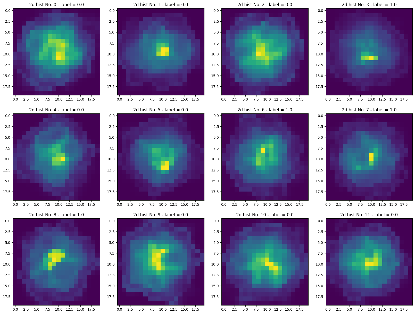
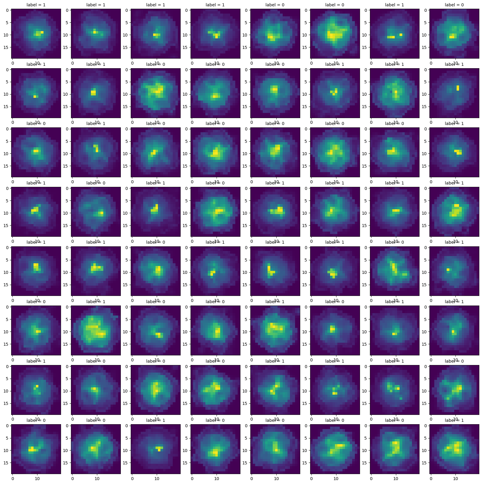
Each collision event is represented as a 20×20 image of the net baryon density distribution in the transverse X–Y plane at fixed time \( t = 3 \, \text{fm}/c \), when fluctuation effects are strongest. These images serve as input to deep learning models for binary classification, distinguishing between spinodal (1) and non-spinodal (Maxwell 0) events.
What is Spinodal Decomposition? (An experimentalist perspective)#
Note: Take this with a grain of salt.
When we collide heavy ions like lead nuclei together at very high energies, we briefly create extreme conditions—very hot and very dense nuclear matter. Under such conditions, the matter may undergo a phase transition of hadronic matter (made of protons and neutrons) possibly turning into quark-gluon plasma .
In these systems, a phase transition can happen smoothly (a crossover) or sharply (first-order) just like ice melting or water boiling. In the case of first-order transitions, there’s often a region where the system becomes unstable, and small fluctuations can grow dramatically.
This unstable region is known as the spinodal region, and the process where small fluctuations in density grow into visible patterns or clumps is called spinodal decomposition.
🕒 Time Evolution in the Spinodal Simulation#
The Spinodal dataset is generated from time-resolved simulations of heavy-ion (Pb+Pb) collisions using UrQMD (Ultra-relativistic Quantum Molecular Dynamics). These simulations model how hot and dense nuclear matter evolves over time, from the moment two nuclei collide to the stage where particles are formed and freeze out.
⏳ How Does the System Evolve?#
The simulation tracks the system through several key stages:
Initial collision (t ≈ 0 fm/c)
Two lead nuclei collide at high energy, compressing and heating nuclear matter.Compression & heating phase
Matter becomes extremely dense and may enter the region of the QCD phase diagram where a first-order phase transition occurs.Passage through the spinodal region
If the equation of state allows it, the system becomes mechanically unstable.
Small density fluctuations grow into visible clumps — this is spinodal decomposition.
Maximal density fluctuation (t = 3 fm/c)
The simulation reaches the moment where clumping patterns are most pronounced.Expansion and freeze-out (later times)
The system expands and cools, eventually forming hadrons (particles like protons and neutrons), which fly out to the detector.
Why It Matters in Nuclear Collisions#
In heavy-ion collisions:
If the system passes through the spinodal region, it might develop clumps of baryons (particles like protons and neutrons).
These clumps are not random—they’re a signature of the phase transition happening out of equilibrium.
Detecting these clumps in simulation is challenging, but they can leave patterns in the spatial distributions of particles.
This is what the Spinodal dataset captures:
Simulated images of net baryon density, where some events have gone through this clumping (spinodal) and others have not (Maxwell – these are thermodynamically stable.)
Our job is to train a neural network to learn the hidden features that distinguish these two cases, just from the images.
So in short, spinodal decomposition is a fingerprint of a violent, out-of-equilibrium transformation of matter, and detecting it could help physicists understand the phase structure of the universe’s most fundamental particles.
This notebook will focus on using Convolutional Neural Networks (CNNs) to classify events from this dataset, illustrating how modern ML techniques can extract subtle physical signatures from event-by-event data.
Loading and preprocessing the data#
For ease of use, I have downloaded the dataset and saved it as a pkl file in the data folder in github.com/cfteach/HUGS2025
!wget https://raw.githubusercontent.com/cfteach/HUGS2025/data/CNN/HUGS2025_CNN_train.pkl
!wget https://raw.githubusercontent.com/cfteach/HUGS2025/data/CNN/HUGS2025_CNN_test.pkl
--2025-06-03 00:04:36--  https://raw.githubusercontent.com/cfteach/HUGS2025/data/CNN/train.pkl
Resolving raw.githubusercontent.com (raw.githubusercontent.com)... 185.199.108.133, 185.199.109.133, 185.199.110.133, ...
Connecting to raw.githubusercontent.com (raw.githubusercontent.com)|185.199.108.133|:443... connected.
HTTP request sent, awaiting response... 404 Not Found
2025-06-03 00:04:36 ERROR 404: Not Found.

--2025-06-03 00:04:36--  https://raw.githubusercontent.com/cfteach/HUGS2025/data/CNN/test.pkl
Resolving raw.githubusercontent.com (raw.githubusercontent.com)... 185.199.108.133, 185.199.109.133, 185.199.110.133, ...
Connecting to raw.githubusercontent.com (raw.githubusercontent.com)|185.199.108.133|:443... connected.
HTTP request sent, awaiting response... 404 Not Found
2025-06-03 00:04:36 ERROR 404: Not Found.
import pickle as pkl
# lets load the data from the pickle files

with open("HUGS2025_CNN_train.pkl", "rb") as f:
    X_train, y_train = pkl.load(f)

with open("HUGS2025_CNN_test.pkl", "rb") as f:
    X_test, y_test = pkl.load(f)
import numpy as np
import torch
import torch.nn as nn
import torch.nn.functional as F
from torch.utils.data import DataLoader, Subset, TensorDataset
device = torch.device("cuda" if torch.cuda.is_available() else "cpu")
print(device)

if device.type == 'cuda':
    print(torch.cuda.get_device_name(0))
else:
  print('cpu')
cuda
Tesla T4
# checking basic content

print (type(X_train))
print (type(y_train))
print (type(X_test))
print (type(y_test))
print(len(X_train))
print(len(X_test))

print(X_train.shape)
print(X_test.shape)

print(y_train.shape)
print(y_test.shape)
<class 'numpy.ndarray'>
<class 'numpy.ndarray'>
<class 'numpy.ndarray'>
<class 'numpy.ndarray'>
20300
8700
(20300, 20, 20)
(8700, 20, 20)
(20300,)
(8700,)
# example 2d histograms
from matplotlib import pyplot as plt
X = X_train
y = y_train

fig, axs = plt.subplots(nrows=3, ncols=4, figsize=(20, 15))
for i, (ax) in enumerate(np.array(axs).ravel()):
    ax.imshow(X[i,:,:])
    ax.set_title('2d hist No. {} - label = {}'.format(i, y[i]))
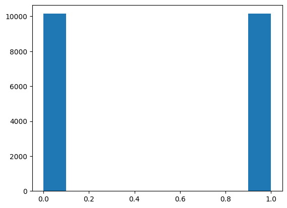
# labels
plt.clf()
plt.hist(y_train, bins = 10)
plt.show()
import torch
from torch.utils.data import TensorDataset, DataLoader, random_split


#y_train_one_hot = F.one_hot(torch.tensor(y_train, dtype = int), num_classes=2).float()
#y_test_one_hot = F.one_hot(torch.tensor(y_test, dtype = int), num_classes=2).float()
if (X_train.ndim == 3):
    X_train = torch.Tensor(X_train).unsqueeze(1)
    X_test = torch.Tensor(X_test).unsqueeze(1)
else:
    X_train = torch.Tensor(X_train)
    X_test = torch.Tensor(X_test)

TRAIN_DATASET = TensorDataset(X_train, torch.tensor(y_train, dtype = int))
test_dataset = TensorDataset(X_test, torch.tensor(y_test, dtype = int))

train_val_split = 0.8
train_val_lengths = [int(len(TRAIN_DATASET)*train_val_split), len(TRAIN_DATASET)-int(len(TRAIN_DATASET)*train_val_split)]
train_dataset, val_dataset = random_split(TRAIN_DATASET, train_val_lengths)

train_loader = DataLoader(train_dataset, batch_size=64, shuffle=True)
val_loader = DataLoader(val_dataset, batch_size=64, shuffle=False)
test_loader = DataLoader(test_dataset, batch_size=64, shuffle=False)

batch_shape = None
# lets test the loaders
for tmpbatch in train_loader:
  print (tmpbatch[0].shape)
  print (tmpbatch[1].shape)
  batch_shape = tmpbatch[0].shape
  # Lets plot the images with labels
  fig, axs = plt.subplots(nrows=8, ncols=8, figsize=(20, 20))
  for i, (ax) in enumerate(np.array(axs).ravel()):
    ax.imshow(tmpbatch[0][i,0,:,:])
    ax.set_title('label = {}'.format(tmpbatch[1][i]), fontsize = 10)
  plt.show()
  break
torch.Size([64, 1, 20, 20])
torch.Size([64])
print(len(train_dataset),len(val_dataset),len(test_dataset))

sample_image, sample_label = train_dataset[0]

print(sample_image.shape, sample_label)

# consistent NCHW format
16240 4060 8700
torch.Size([1, 20, 20]) tensor(1)
Constructing a CNN in PyTorch#
import torch
import torch.nn as nn
import torch.nn.functional as F

import torch
import torch.nn as nn
import torch.nn.functional as F

def get_trainable_params(model):
    return sum(p.numel() for p in model.parameters() if p.requires_grad)

class SpinodalCNN(nn.Module):
    def __init__(self, input_shape=(1, 20, 20)):
        super(SpinodalCNN, self).__init__()

        # Convolutional layers
        self.conv1 = nn.Conv2d(1, 15, kernel_size=3, padding=1)  # "same" padding
        self.conv2 = nn.Conv2d(15, 15, kernel_size=3, padding=1)
        self.pool1 = nn.MaxPool2d(kernel_size=2)

        self.conv3 = nn.Conv2d(15, 25, kernel_size=3, padding=1)
        self.pool2 = nn.MaxPool2d(kernel_size=2)

        self.dropout = nn.Dropout(0.4)

        # Flattened size (computed once using dummy input)
        self.flattened_size = self._get_flattened_size(input_shape)

        # Fully connected layers
        self.fc1 = nn.Linear(self.flattened_size, 10)
        self.fc2 = nn.Linear(10, 1)

    def _get_flattened_size(self, input_shape):
        with torch.no_grad():
            dummy = torch.zeros(1, *input_shape)
            x = F.relu(self.conv1(dummy))
            x = F.relu(self.conv2(x))
            x = self.pool1(x)
            x = F.relu(self.conv3(x))
            x = self.pool2(x)
            return x.view(1, -1).size(1)

    def forward(self, x):
        x = F.relu(self.conv1(x))
        x = F.relu(self.conv2(x))
        x = self.pool1(x)
        x = F.relu(self.conv3(x))
        x = self.pool2(x)
        x = self.dropout(x)
        x = x.view(x.size(0), -1)  # Flatten
        x = F.relu(self.fc1(x))
        x = torch.sigmoid(self.fc2(x))  # For BCELoss
        return x

device = torch.device("cuda" if torch.cuda.is_available() else "cpu")

model = SpinodalCNN()
model = model.to(device)
print (model)
print (f'Model has {get_trainable_params(model):.2e} trainable parameters')
print (f"Model is on {device}")
SpinodalCNN(
  (conv1): Conv2d(1, 15, kernel_size=(3, 3), stride=(1, 1), padding=(1, 1))
  (conv2): Conv2d(15, 15, kernel_size=(3, 3), stride=(1, 1), padding=(1, 1))
  (pool1): MaxPool2d(kernel_size=2, stride=2, padding=0, dilation=1, ceil_mode=False)
  (conv3): Conv2d(15, 25, kernel_size=(3, 3), stride=(1, 1), padding=(1, 1))
  (pool2): MaxPool2d(kernel_size=2, stride=2, padding=0, dilation=1, ceil_mode=False)
  (dropout): Dropout(p=0.4, inplace=False)
  (fc1): Linear(in_features=625, out_features=10, bias=True)
  (fc2): Linear(in_features=10, out_features=1, bias=True)
)
Model has 1.19e+04 trainable parameters
Model is on cuda
# Lets try compute input for train

for tmpx, tmpy in train_loader:
  tmpx = tmpx.to(device)
  tmpy = tmpy.to(device)
  print(f"input shape is {tmpx.shape}, and output shape is {model(tmpx.float()).shape}")
  break
input shape is torch.Size([64, 1, 20, 20]), and output shape is torch.Size([64, 1])
import torch
import torch.nn as nn
import torch.optim as optim
from torch.utils.data import DataLoader

def train_spinodal_cnn(model, train_loader, val_loader=None,
                       epochs=5, lr=1e-3, start = 0,
                       device='cuda' if torch.cuda.is_available() else 'cpu',
                       metrics = None
                       ):
    if metrics is None:
        metrics = {
            'train_loss': [],
            'train_acc': [],
            'val_loss': [],
            'val_acc': []
        }
    model.to(device)
    criterion = nn.BCELoss()
    optimizer = optim.Adam(model.parameters(), lr=lr)

    for epoch in range(start, start + epochs):
        model.train()
        running_loss, correct, total = 0.0, 0, 0

        for inputs, labels in train_loader:
            inputs, labels = inputs.to(device).float(), labels.to(device).float().unsqueeze(1)

            optimizer.zero_grad()
            outputs = model(inputs)  # sigmoid outputs in [0,1]
            loss = criterion(outputs, labels)
            loss.backward()
            optimizer.step()

            # Track stats
            running_loss += loss.item() * inputs.size(0)
            preds = (outputs > 0.5).float()
            correct += (preds == labels).sum().item()
            total += labels.size(0)

        avg_loss = running_loss / total
        acc = correct / total * 100
        print(f"[Epoch {epoch+1:02d}] Train Loss: {avg_loss:.4f} | Train Acc: {acc:.2f}%")
        metrics['train_loss'].append(avg_loss)
        metrics['train_acc'].append(acc)

        # Optional validation
        if val_loader:
            model.eval()
            val_loss, val_correct, val_total = 0.0, 0, 0
            with torch.no_grad():
                for inputs, labels in val_loader:
                    inputs, labels = inputs.to(device).float(), labels.to(device).float().unsqueeze(1)

                    outputs = model(inputs)
                    loss = criterion(outputs, labels)

                    val_loss += loss.item() * inputs.size(0)
                    preds = (outputs > 0.5).float()
                    val_correct += (preds == labels).sum().item()
                    val_total += labels.size(0)

            avg_val_loss = val_loss / val_total
            val_acc = val_correct / val_total * 100
            print(f"              Val Loss:   {avg_val_loss:.4f} | Val Acc:   {val_acc:.2f}%")
            metrics['val_loss'].append(avg_val_loss)
            metrics['val_acc'].append(val_acc)

    return (model, metrics)
try:
    start = len(metrics['train_loss'])
    metrics = metrics
except:
    start = 0
    metrics = None
trained_model, metrics = train_spinodal_cnn(model, train_loader, val_loader, epochs=25, start = start, metrics= metrics, device=device)
[Epoch 01] Train Loss: 0.5110 | Train Acc: 75.02%
              Val Loss:   0.4469 | Val Acc:   80.00%
[Epoch 02] Train Loss: 0.4622 | Train Acc: 79.19%
              Val Loss:   0.4612 | Val Acc:   78.60%
[Epoch 03] Train Loss: 0.4534 | Train Acc: 79.62%
              Val Loss:   0.4366 | Val Acc:   80.49%
[Epoch 04] Train Loss: 0.4446 | Train Acc: 80.18%
              Val Loss:   0.4400 | Val Acc:   80.20%
[Epoch 05] Train Loss: 0.4396 | Train Acc: 80.54%
              Val Loss:   0.4292 | Val Acc:   80.84%
[Epoch 06] Train Loss: 0.4341 | Train Acc: 80.81%
              Val Loss:   0.4108 | Val Acc:   81.95%
[Epoch 07] Train Loss: 0.4230 | Train Acc: 81.32%
              Val Loss:   0.4504 | Val Acc:   79.63%
[Epoch 08] Train Loss: 0.4174 | Train Acc: 81.77%
              Val Loss:   0.3980 | Val Acc:   82.59%
[Epoch 09] Train Loss: 0.4096 | Train Acc: 82.51%
              Val Loss:   0.4098 | Val Acc:   82.39%
[Epoch 10] Train Loss: 0.3980 | Train Acc: 83.06%
              Val Loss:   0.4101 | Val Acc:   81.82%
[Epoch 11] Train Loss: 0.3991 | Train Acc: 82.84%
              Val Loss:   0.3870 | Val Acc:   82.86%
[Epoch 12] Train Loss: 0.3916 | Train Acc: 83.31%
              Val Loss:   0.3905 | Val Acc:   82.83%
[Epoch 13] Train Loss: 0.3831 | Train Acc: 83.73%
              Val Loss:   0.3644 | Val Acc:   84.80%
[Epoch 14] Train Loss: 0.3771 | Train Acc: 84.33%
              Val Loss:   0.3560 | Val Acc:   85.07%
[Epoch 15] Train Loss: 0.3696 | Train Acc: 84.64%
              Val Loss:   0.3632 | Val Acc:   84.63%
[Epoch 16] Train Loss: 0.3695 | Train Acc: 84.43%
              Val Loss:   0.3502 | Val Acc:   84.93%
[Epoch 17] Train Loss: 0.3611 | Train Acc: 84.70%
              Val Loss:   0.3332 | Val Acc:   86.03%
[Epoch 18] Train Loss: 0.3585 | Train Acc: 85.01%
              Val Loss:   0.3491 | Val Acc:   85.39%
[Epoch 19] Train Loss: 0.3454 | Train Acc: 85.57%
              Val Loss:   0.3277 | Val Acc:   86.50%
[Epoch 20] Train Loss: 0.3475 | Train Acc: 85.43%
              Val Loss:   0.3197 | Val Acc:   86.43%
[Epoch 21] Train Loss: 0.3410 | Train Acc: 85.82%
              Val Loss:   0.3163 | Val Acc:   86.90%
[Epoch 22] Train Loss: 0.3394 | Train Acc: 85.92%
              Val Loss:   0.3289 | Val Acc:   85.81%
[Epoch 23] Train Loss: 0.3313 | Train Acc: 86.16%
              Val Loss:   0.3099 | Val Acc:   87.02%
[Epoch 24] Train Loss: 0.3244 | Train Acc: 86.45%
              Val Loss:   0.3345 | Val Acc:   85.57%
[Epoch 25] Train Loss: 0.3261 | Train Acc: 86.23%
              Val Loss:   0.3196 | Val Acc:   85.99%
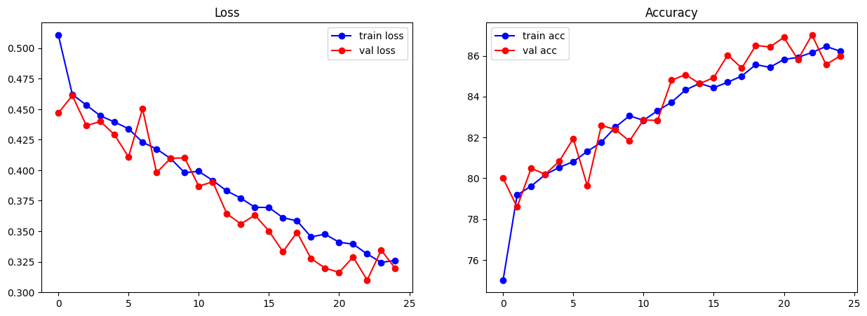
import matplotlib.pyplot as plt

# lets plots the metrics
fig, ax= plt.subplots(nrows = 1, ncols = 2, figsize = (15, 5))
ax[0].plot(metrics['train_loss'], 'bo-', label = 'train loss')
ax[0].plot(metrics['val_loss'], 'ro-', label = 'val loss')
ax[0].set_title('Loss')
ax[0].legend()
ax[1].plot(metrics['train_acc'], 'bo-', label = 'train acc')
ax[1].plot(metrics['val_acc'], 'ro-', label = 'val acc')
ax[1].set_title('Accuracy')
ax[1].legend()
plt.show()
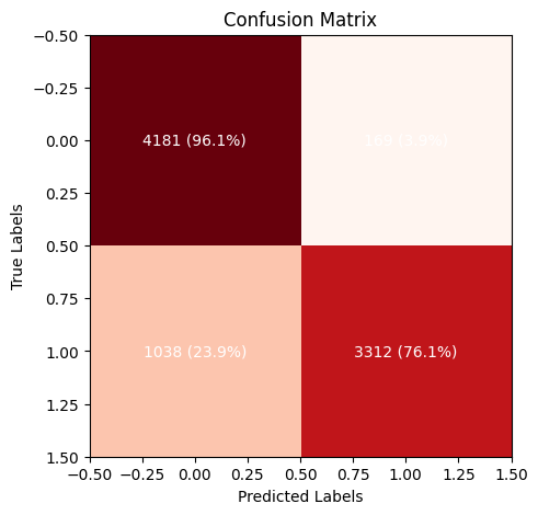
# Lets now test on test data and plot confusion metric as well. Also plot the ROC curve
from sklearn.metrics import confusion_matrix, roc_curve
y_pred = []
y_true = []
with torch.no_grad():
for inputs, labels in test_loader:
inputs, labels = inputs.to(device).float(), labels.to(device).float().unsqueeze(1)
outputs = model(inputs)
y_pred.extend(outputs.cpu().numpy())
y_true.extend(labels.cpu().numpy())
y_pred = np.array(y_pred)
y_true = np.array(y_true)
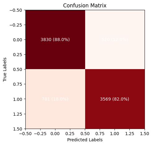
# lets compute confusion metric and ROC curve
cm = confusion_matrix(y_true, y_pred > 0.5)
# Plot the confusion matrix
fig, ax = plt.subplots(figsize=(5, 5))
ax.imshow(cm, interpolation='nearest', cmap=plt.cm.Reds)
# put the percentage in each cell
for i in range(cm.shape[0]):
for j in range(cm.shape[1]):
ax.text(j, i, f'{cm[i, j]} ({cm[i, j]/np.sum(cm[i, :])*100:.1f}%)', ha='center', va='center', color='white')
ax.set_title('Confusion Matrix')
ax.set_xlabel('Predicted Labels')
ax.set_ylabel('True Labels')
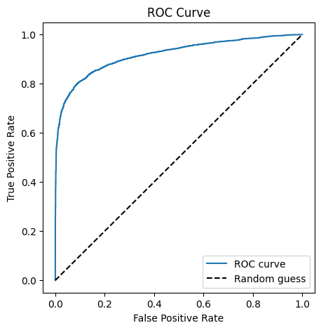
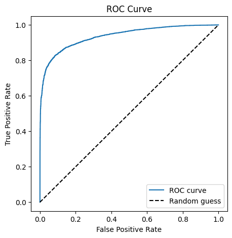
# lets plot the ROC curve
fpr, tpr, _ = roc_curve(y_true, y_pred)
plt.figure(figsize=(5, 5))
plt.plot(fpr, tpr, label='ROC curve')
plt.plot([0, 1], [0, 1], 'k--', label='Random guess')
plt.xlabel('False Positive Rate')
plt.ylabel('True Positive Rate')
plt.title('ROC Curve')
plt.legend()
plt.show()
Introduction to Fine-Tuning a CNN#
Now that we’ve prepared our dataset and constructed appropriate data loaders, it’s time to train a Convolutional Neural Network (CNN). However, rather than training a model entirely from scratch—which requires large amounts of data and compute—we’ll adopt a more efficient approach known as fine-tuning.
Fine-tuning leverages a pretrained model—a model that has already learned useful image features by training on a large and diverse dataset, such as ImageNet, which contains over a million labeled images across 1,000 categories. The key idea is to transfer this prior knowledge to a new task, using a smaller, domain-specific dataset.
Why Use a Pretrained Model?#
CNNs trained on large datasets like ImageNet learn to detect general visual patterns in their early layers—such as edges, gradients, and textures—that are useful for a wide range of vision tasks. These general-purpose features form the backbone of the model. By reusing them, we:
Reduce training time.
Require less data to achieve good performance.
Improve generalization.
How Does Fine-Tuning Work?#
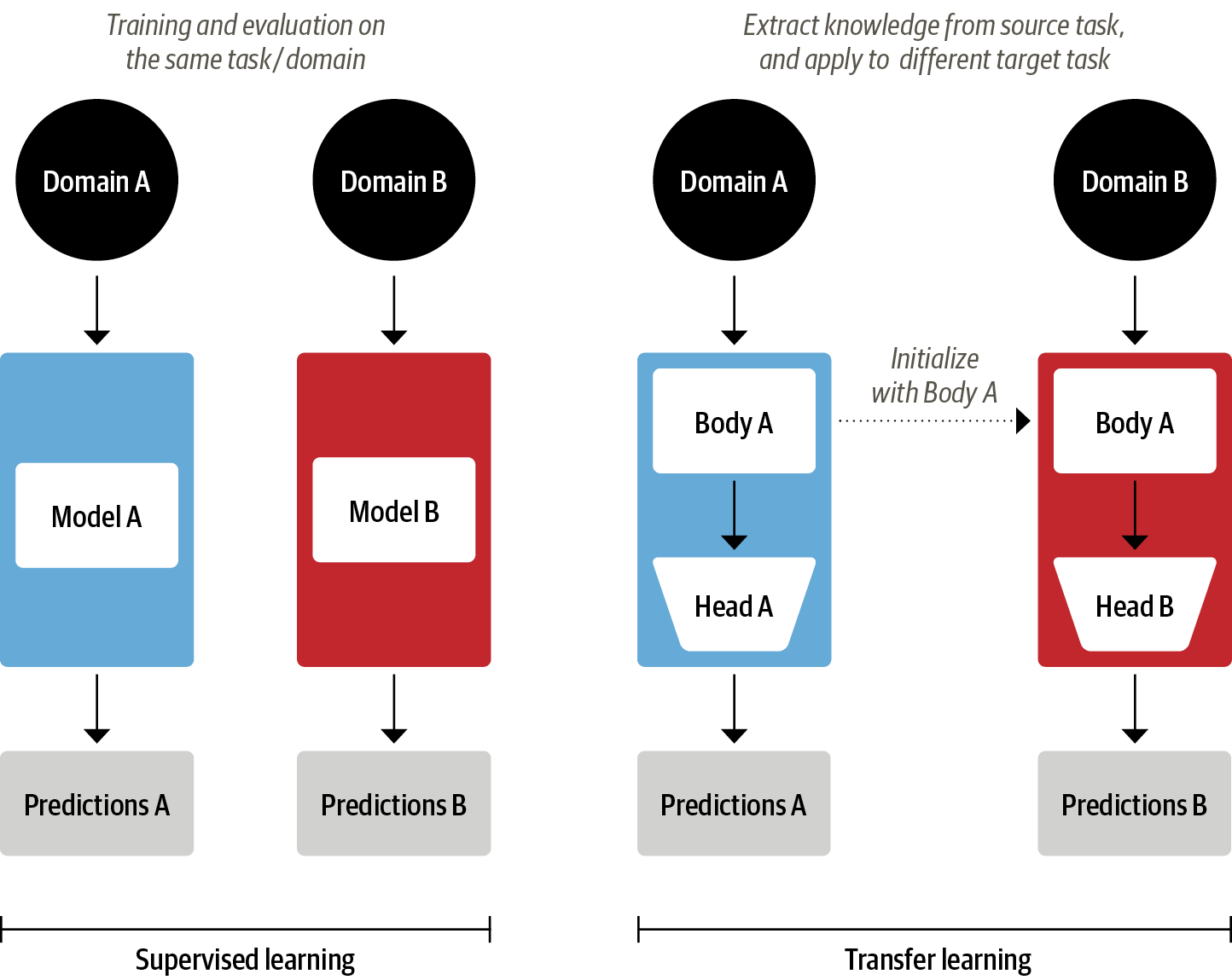
In practice, we perform transfer learning in two main steps:
Replace the classifier head: Since our target task (e.g., classifying spinodal vs. Maxwell events) may have a different number of output classes than ImageNet, we discard the final classification layer (originally designed for 1,000 ImageNet classes) and replace it with a new, randomly initialized layer appropriate for our task (e.g., 2-class binary classification).
Adapt the model:
In feature extraction mode, we freeze all pretrained layers and train only the new head.
In fine-tuning mode, we allow some or all of the pretrained layers to update during training, letting the model adapt to the new dataset.
This approach is particularly effective when we have a small dataset and when the domain shares visual characteristics with natural images.
Summary#
This strategy—reusing pretrained weights and adapting the model to a new task—is broadly referred to as transfer learning, and is a cornerstone of modern deep learning in fields ranging from computer vision and natural language processing to scientific data analysis.
# Let us look into all the models torchvision has to offer
from torchvision import models
# https://docs.pytorch.org/vision/0.9/models.html
# List all available models
all_models = models.list_models()

for idx, name in enumerate(all_models):
    print (f"{idx+1}. {name}")
1. alexnet
2. convnext_base
3. convnext_large
4. convnext_small
5. convnext_tiny
6. deeplabv3_mobilenet_v3_large
7. deeplabv3_resnet101
8. deeplabv3_resnet50
9. densenet121
10. densenet161
11. densenet169
12. densenet201
13. efficientnet_b0
14. efficientnet_b1
15. efficientnet_b2
16. efficientnet_b3
17. efficientnet_b4
18. efficientnet_b5
19. efficientnet_b6
20. efficientnet_b7
21. efficientnet_v2_l
22. efficientnet_v2_m
23. efficientnet_v2_s
24. fasterrcnn_mobilenet_v3_large_320_fpn
25. fasterrcnn_mobilenet_v3_large_fpn
26. fasterrcnn_resnet50_fpn
27. fasterrcnn_resnet50_fpn_v2
28. fcn_resnet101
29. fcn_resnet50
30. fcos_resnet50_fpn
31. googlenet
32. inception_v3
33. keypointrcnn_resnet50_fpn
34. lraspp_mobilenet_v3_large
35. maskrcnn_resnet50_fpn
36. maskrcnn_resnet50_fpn_v2
37. maxvit_t
38. mc3_18
39. mnasnet0_5
40. mnasnet0_75
41. mnasnet1_0
42. mnasnet1_3
43. mobilenet_v2
44. mobilenet_v3_large
45. mobilenet_v3_small
46. mvit_v1_b
47. mvit_v2_s
48. quantized_googlenet
49. quantized_inception_v3
50. quantized_mobilenet_v2
51. quantized_mobilenet_v3_large
52. quantized_resnet18
53. quantized_resnet50
54. quantized_resnext101_32x8d
55. quantized_resnext101_64x4d
56. quantized_shufflenet_v2_x0_5
57. quantized_shufflenet_v2_x1_0
58. quantized_shufflenet_v2_x1_5
59. quantized_shufflenet_v2_x2_0
60. r2plus1d_18
61. r3d_18
62. raft_large
63. raft_small
64. regnet_x_16gf
65. regnet_x_1_6gf
66. regnet_x_32gf
67. regnet_x_3_2gf
68. regnet_x_400mf
69. regnet_x_800mf
70. regnet_x_8gf
71. regnet_y_128gf
72. regnet_y_16gf
73. regnet_y_1_6gf
74. regnet_y_32gf
75. regnet_y_3_2gf
76. regnet_y_400mf
77. regnet_y_800mf
78. regnet_y_8gf
79. resnet101
80. resnet152
81. resnet18
82. resnet34
83. resnet50
84. resnext101_32x8d
85. resnext101_64x4d
86. resnext50_32x4d
87. retinanet_resnet50_fpn
88. retinanet_resnet50_fpn_v2
89. s3d
90. shufflenet_v2_x0_5
91. shufflenet_v2_x1_0
92. shufflenet_v2_x1_5
93. shufflenet_v2_x2_0
94. squeezenet1_0
95. squeezenet1_1
96. ssd300_vgg16
97. ssdlite320_mobilenet_v3_large
98. swin3d_b
99. swin3d_s
100. swin3d_t
101. swin_b
102. swin_s
103. swin_t
104. swin_v2_b
105. swin_v2_s
106. swin_v2_t
107. vgg11
108. vgg11_bn
109. vgg13
110. vgg13_bn
111. vgg16
112. vgg16_bn
113. vgg19
114. vgg19_bn
115. vit_b_16
116. vit_b_32
117. vit_h_14
118. vit_l_16
119. vit_l_32
120. wide_resnet101_2
121. wide_resnet50_2
What is MobileNet?#
MobileNet is a family of lightweight convolutional neural networks designed for efficient inference on mobile and embedded devices. Introduced by Google, MobileNet achieves high accuracy while maintaining a low computational footprint, making it ideal for applications where resources are limited.
MobileNet is built using a key architectural innovation called depthwise separable convolutions, which factorize a standard convolution into two operations:
A depthwise convolution, which applies a single filter per input channel.
A pointwise convolution (1×1 convolution), which linearly combines the outputs of the depthwise layer.
This factorization drastically reduces the number of parameters and computational cost, compared to standard convolutions, without a significant loss in accuracy.
MobileNet models are typically pretrained on the ImageNet dataset, which contains over 1.2 million images across 1,000 classes. Through this large-scale training, the network learns rich and general-purpose visual features such as edges, textures, and object parts. These learned weights are then transferred and fine-tuned on domain-specific datasets (like our spinodal classification images) to enable accurate and efficient task-specific models.
mobileNet = models.mobilenet_v2(weights = models.MobileNet_V2_Weights.DEFAULT)

print (mobileNet)
Downloading: "https://download.pytorch.org/models/mobilenet_v2-7ebf99e0.pth" to /root/.cache/torch/hub/checkpoints/mobilenet_v2-7ebf99e0.pth
100%|██████████| 13.6M/13.6M [00:00<00:00, 154MB/s]
MobileNetV2(
  (features): Sequential(
    (0): Conv2dNormActivation(
      (0): Conv2d(3, 32, kernel_size=(3, 3), stride=(2, 2), padding=(1, 1), bias=False)
      (1): BatchNorm2d(32, eps=1e-05, momentum=0.1, affine=True, track_running_stats=True)
      (2): ReLU6(inplace=True)
    )
    (1): InvertedResidual(
      (conv): Sequential(
        (0): Conv2dNormActivation(
          (0): Conv2d(32, 32, kernel_size=(3, 3), stride=(1, 1), padding=(1, 1), groups=32, bias=False)
          (1): BatchNorm2d(32, eps=1e-05, momentum=0.1, affine=True, track_running_stats=True)
          (2): ReLU6(inplace=True)
        )
        (1): Conv2d(32, 16, kernel_size=(1, 1), stride=(1, 1), bias=False)
        (2): BatchNorm2d(16, eps=1e-05, momentum=0.1, affine=True, track_running_stats=True)
      )
    )
    (2): InvertedResidual(
      (conv): Sequential(
        (0): Conv2dNormActivation(
          (0): Conv2d(16, 96, kernel_size=(1, 1), stride=(1, 1), bias=False)
          (1): BatchNorm2d(96, eps=1e-05, momentum=0.1, affine=True, track_running_stats=True)
          (2): ReLU6(inplace=True)
        )
        (1): Conv2dNormActivation(
          (0): Conv2d(96, 96, kernel_size=(3, 3), stride=(2, 2), padding=(1, 1), groups=96, bias=False)
          (1): BatchNorm2d(96, eps=1e-05, momentum=0.1, affine=True, track_running_stats=True)
          (2): ReLU6(inplace=True)
        )
        (2): Conv2d(96, 24, kernel_size=(1, 1), stride=(1, 1), bias=False)
        (3): BatchNorm2d(24, eps=1e-05, momentum=0.1, affine=True, track_running_stats=True)
      )
    )
    (3): InvertedResidual(
      (conv): Sequential(
        (0): Conv2dNormActivation(
          (0): Conv2d(24, 144, kernel_size=(1, 1), stride=(1, 1), bias=False)
          (1): BatchNorm2d(144, eps=1e-05, momentum=0.1, affine=True, track_running_stats=True)
          (2): ReLU6(inplace=True)
        )
        (1): Conv2dNormActivation(
          (0): Conv2d(144, 144, kernel_size=(3, 3), stride=(1, 1), padding=(1, 1), groups=144, bias=False)
          (1): BatchNorm2d(144, eps=1e-05, momentum=0.1, affine=True, track_running_stats=True)
          (2): ReLU6(inplace=True)
        )
        (2): Conv2d(144, 24, kernel_size=(1, 1), stride=(1, 1), bias=False)
        (3): BatchNorm2d(24, eps=1e-05, momentum=0.1, affine=True, track_running_stats=True)
      )
    )
    (4): InvertedResidual(
      (conv): Sequential(
        (0): Conv2dNormActivation(
          (0): Conv2d(24, 144, kernel_size=(1, 1), stride=(1, 1), bias=False)
          (1): BatchNorm2d(144, eps=1e-05, momentum=0.1, affine=True, track_running_stats=True)
          (2): ReLU6(inplace=True)
        )
        (1): Conv2dNormActivation(
          (0): Conv2d(144, 144, kernel_size=(3, 3), stride=(2, 2), padding=(1, 1), groups=144, bias=False)
          (1): BatchNorm2d(144, eps=1e-05, momentum=0.1, affine=True, track_running_stats=True)
          (2): ReLU6(inplace=True)
        )
        (2): Conv2d(144, 32, kernel_size=(1, 1), stride=(1, 1), bias=False)
        (3): BatchNorm2d(32, eps=1e-05, momentum=0.1, affine=True, track_running_stats=True)
      )
    )
    (5): InvertedResidual(
      (conv): Sequential(
        (0): Conv2dNormActivation(
          (0): Conv2d(32, 192, kernel_size=(1, 1), stride=(1, 1), bias=False)
          (1): BatchNorm2d(192, eps=1e-05, momentum=0.1, affine=True, track_running_stats=True)
          (2): ReLU6(inplace=True)
        )
        (1): Conv2dNormActivation(
          (0): Conv2d(192, 192, kernel_size=(3, 3), stride=(1, 1), padding=(1, 1), groups=192, bias=False)
          (1): BatchNorm2d(192, eps=1e-05, momentum=0.1, affine=True, track_running_stats=True)
          (2): ReLU6(inplace=True)
        )
        (2): Conv2d(192, 32, kernel_size=(1, 1), stride=(1, 1), bias=False)
        (3): BatchNorm2d(32, eps=1e-05, momentum=0.1, affine=True, track_running_stats=True)
      )
    )
    (6): InvertedResidual(
      (conv): Sequential(
        (0): Conv2dNormActivation(
          (0): Conv2d(32, 192, kernel_size=(1, 1), stride=(1, 1), bias=False)
          (1): BatchNorm2d(192, eps=1e-05, momentum=0.1, affine=True, track_running_stats=True)
          (2): ReLU6(inplace=True)
        )
        (1): Conv2dNormActivation(
          (0): Conv2d(192, 192, kernel_size=(3, 3), stride=(1, 1), padding=(1, 1), groups=192, bias=False)
          (1): BatchNorm2d(192, eps=1e-05, momentum=0.1, affine=True, track_running_stats=True)
          (2): ReLU6(inplace=True)
        )
        (2): Conv2d(192, 32, kernel_size=(1, 1), stride=(1, 1), bias=False)
        (3): BatchNorm2d(32, eps=1e-05, momentum=0.1, affine=True, track_running_stats=True)
      )
    )
    (7): InvertedResidual(
      (conv): Sequential(
        (0): Conv2dNormActivation(
          (0): Conv2d(32, 192, kernel_size=(1, 1), stride=(1, 1), bias=False)
          (1): BatchNorm2d(192, eps=1e-05, momentum=0.1, affine=True, track_running_stats=True)
          (2): ReLU6(inplace=True)
        )
        (1): Conv2dNormActivation(
          (0): Conv2d(192, 192, kernel_size=(3, 3), stride=(2, 2), padding=(1, 1), groups=192, bias=False)
          (1): BatchNorm2d(192, eps=1e-05, momentum=0.1, affine=True, track_running_stats=True)
          (2): ReLU6(inplace=True)
        )
        (2): Conv2d(192, 64, kernel_size=(1, 1), stride=(1, 1), bias=False)
        (3): BatchNorm2d(64, eps=1e-05, momentum=0.1, affine=True, track_running_stats=True)
      )
    )
    (8): InvertedResidual(
      (conv): Sequential(
        (0): Conv2dNormActivation(
          (0): Conv2d(64, 384, kernel_size=(1, 1), stride=(1, 1), bias=False)
          (1): BatchNorm2d(384, eps=1e-05, momentum=0.1, affine=True, track_running_stats=True)
          (2): ReLU6(inplace=True)
        )
        (1): Conv2dNormActivation(
          (0): Conv2d(384, 384, kernel_size=(3, 3), stride=(1, 1), padding=(1, 1), groups=384, bias=False)
          (1): BatchNorm2d(384, eps=1e-05, momentum=0.1, affine=True, track_running_stats=True)
          (2): ReLU6(inplace=True)
        )
        (2): Conv2d(384, 64, kernel_size=(1, 1), stride=(1, 1), bias=False)
        (3): BatchNorm2d(64, eps=1e-05, momentum=0.1, affine=True, track_running_stats=True)
      )
    )
    (9): InvertedResidual(
      (conv): Sequential(
        (0): Conv2dNormActivation(
          (0): Conv2d(64, 384, kernel_size=(1, 1), stride=(1, 1), bias=False)
          (1): BatchNorm2d(384, eps=1e-05, momentum=0.1, affine=True, track_running_stats=True)
          (2): ReLU6(inplace=True)
        )
        (1): Conv2dNormActivation(
          (0): Conv2d(384, 384, kernel_size=(3, 3), stride=(1, 1), padding=(1, 1), groups=384, bias=False)
          (1): BatchNorm2d(384, eps=1e-05, momentum=0.1, affine=True, track_running_stats=True)
          (2): ReLU6(inplace=True)
        )
        (2): Conv2d(384, 64, kernel_size=(1, 1), stride=(1, 1), bias=False)
        (3): BatchNorm2d(64, eps=1e-05, momentum=0.1, affine=True, track_running_stats=True)
      )
    )
    (10): InvertedResidual(
      (conv): Sequential(
        (0): Conv2dNormActivation(
          (0): Conv2d(64, 384, kernel_size=(1, 1), stride=(1, 1), bias=False)
          (1): BatchNorm2d(384, eps=1e-05, momentum=0.1, affine=True, track_running_stats=True)
          (2): ReLU6(inplace=True)
        )
        (1): Conv2dNormActivation(
          (0): Conv2d(384, 384, kernel_size=(3, 3), stride=(1, 1), padding=(1, 1), groups=384, bias=False)
          (1): BatchNorm2d(384, eps=1e-05, momentum=0.1, affine=True, track_running_stats=True)
          (2): ReLU6(inplace=True)
        )
        (2): Conv2d(384, 64, kernel_size=(1, 1), stride=(1, 1), bias=False)
        (3): BatchNorm2d(64, eps=1e-05, momentum=0.1, affine=True, track_running_stats=True)
      )
    )
    (11): InvertedResidual(
      (conv): Sequential(
        (0): Conv2dNormActivation(
          (0): Conv2d(64, 384, kernel_size=(1, 1), stride=(1, 1), bias=False)
          (1): BatchNorm2d(384, eps=1e-05, momentum=0.1, affine=True, track_running_stats=True)
          (2): ReLU6(inplace=True)
        )
        (1): Conv2dNormActivation(
          (0): Conv2d(384, 384, kernel_size=(3, 3), stride=(1, 1), padding=(1, 1), groups=384, bias=False)
          (1): BatchNorm2d(384, eps=1e-05, momentum=0.1, affine=True, track_running_stats=True)
          (2): ReLU6(inplace=True)
        )
        (2): Conv2d(384, 96, kernel_size=(1, 1), stride=(1, 1), bias=False)
        (3): BatchNorm2d(96, eps=1e-05, momentum=0.1, affine=True, track_running_stats=True)
      )
    )
    (12): InvertedResidual(
      (conv): Sequential(
        (0): Conv2dNormActivation(
          (0): Conv2d(96, 576, kernel_size=(1, 1), stride=(1, 1), bias=False)
          (1): BatchNorm2d(576, eps=1e-05, momentum=0.1, affine=True, track_running_stats=True)
          (2): ReLU6(inplace=True)
        )
        (1): Conv2dNormActivation(
          (0): Conv2d(576, 576, kernel_size=(3, 3), stride=(1, 1), padding=(1, 1), groups=576, bias=False)
          (1): BatchNorm2d(576, eps=1e-05, momentum=0.1, affine=True, track_running_stats=True)
          (2): ReLU6(inplace=True)
        )
        (2): Conv2d(576, 96, kernel_size=(1, 1), stride=(1, 1), bias=False)
        (3): BatchNorm2d(96, eps=1e-05, momentum=0.1, affine=True, track_running_stats=True)
      )
    )
    (13): InvertedResidual(
      (conv): Sequential(
        (0): Conv2dNormActivation(
          (0): Conv2d(96, 576, kernel_size=(1, 1), stride=(1, 1), bias=False)
          (1): BatchNorm2d(576, eps=1e-05, momentum=0.1, affine=True, track_running_stats=True)
          (2): ReLU6(inplace=True)
        )
        (1): Conv2dNormActivation(
          (0): Conv2d(576, 576, kernel_size=(3, 3), stride=(1, 1), padding=(1, 1), groups=576, bias=False)
          (1): BatchNorm2d(576, eps=1e-05, momentum=0.1, affine=True, track_running_stats=True)
          (2): ReLU6(inplace=True)
        )
        (2): Conv2d(576, 96, kernel_size=(1, 1), stride=(1, 1), bias=False)
        (3): BatchNorm2d(96, eps=1e-05, momentum=0.1, affine=True, track_running_stats=True)
      )
    )
    (14): InvertedResidual(
      (conv): Sequential(
        (0): Conv2dNormActivation(
          (0): Conv2d(96, 576, kernel_size=(1, 1), stride=(1, 1), bias=False)
          (1): BatchNorm2d(576, eps=1e-05, momentum=0.1, affine=True, track_running_stats=True)
          (2): ReLU6(inplace=True)
        )
        (1): Conv2dNormActivation(
          (0): Conv2d(576, 576, kernel_size=(3, 3), stride=(2, 2), padding=(1, 1), groups=576, bias=False)
          (1): BatchNorm2d(576, eps=1e-05, momentum=0.1, affine=True, track_running_stats=True)
          (2): ReLU6(inplace=True)
        )
        (2): Conv2d(576, 160, kernel_size=(1, 1), stride=(1, 1), bias=False)
        (3): BatchNorm2d(160, eps=1e-05, momentum=0.1, affine=True, track_running_stats=True)
      )
    )
    (15): InvertedResidual(
      (conv): Sequential(
        (0): Conv2dNormActivation(
          (0): Conv2d(160, 960, kernel_size=(1, 1), stride=(1, 1), bias=False)
          (1): BatchNorm2d(960, eps=1e-05, momentum=0.1, affine=True, track_running_stats=True)
          (2): ReLU6(inplace=True)
        )
        (1): Conv2dNormActivation(
          (0): Conv2d(960, 960, kernel_size=(3, 3), stride=(1, 1), padding=(1, 1), groups=960, bias=False)
          (1): BatchNorm2d(960, eps=1e-05, momentum=0.1, affine=True, track_running_stats=True)
          (2): ReLU6(inplace=True)
        )
        (2): Conv2d(960, 160, kernel_size=(1, 1), stride=(1, 1), bias=False)
        (3): BatchNorm2d(160, eps=1e-05, momentum=0.1, affine=True, track_running_stats=True)
      )
    )
    (16): InvertedResidual(
      (conv): Sequential(
        (0): Conv2dNormActivation(
          (0): Conv2d(160, 960, kernel_size=(1, 1), stride=(1, 1), bias=False)
          (1): BatchNorm2d(960, eps=1e-05, momentum=0.1, affine=True, track_running_stats=True)
          (2): ReLU6(inplace=True)
        )
        (1): Conv2dNormActivation(
          (0): Conv2d(960, 960, kernel_size=(3, 3), stride=(1, 1), padding=(1, 1), groups=960, bias=False)
          (1): BatchNorm2d(960, eps=1e-05, momentum=0.1, affine=True, track_running_stats=True)
          (2): ReLU6(inplace=True)
        )
        (2): Conv2d(960, 160, kernel_size=(1, 1), stride=(1, 1), bias=False)
        (3): BatchNorm2d(160, eps=1e-05, momentum=0.1, affine=True, track_running_stats=True)
      )
    )
    (17): InvertedResidual(
      (conv): Sequential(
        (0): Conv2dNormActivation(
          (0): Conv2d(160, 960, kernel_size=(1, 1), stride=(1, 1), bias=False)
          (1): BatchNorm2d(960, eps=1e-05, momentum=0.1, affine=True, track_running_stats=True)
          (2): ReLU6(inplace=True)
        )
        (1): Conv2dNormActivation(
          (0): Conv2d(960, 960, kernel_size=(3, 3), stride=(1, 1), padding=(1, 1), groups=960, bias=False)
          (1): BatchNorm2d(960, eps=1e-05, momentum=0.1, affine=True, track_running_stats=True)
          (2): ReLU6(inplace=True)
        )
        (2): Conv2d(960, 320, kernel_size=(1, 1), stride=(1, 1), bias=False)
        (3): BatchNorm2d(320, eps=1e-05, momentum=0.1, affine=True, track_running_stats=True)
      )
    )
    (18): Conv2dNormActivation(
      (0): Conv2d(320, 1280, kernel_size=(1, 1), stride=(1, 1), bias=False)
      (1): BatchNorm2d(1280, eps=1e-05, momentum=0.1, affine=True, track_running_stats=True)
      (2): ReLU6(inplace=True)
    )
  )
  (classifier): Sequential(
    (0): Dropout(p=0.2, inplace=False)
    (1): Linear(in_features=1280, out_features=1000, bias=True)
  )
)
for name, param in mobileNet.named_parameters():
    print (name, param.shape)
features.0.0.weight torch.Size([32, 3, 3, 3])
features.0.1.weight torch.Size([32])
features.0.1.bias torch.Size([32])
features.1.conv.0.0.weight torch.Size([32, 1, 3, 3])
features.1.conv.0.1.weight torch.Size([32])
features.1.conv.0.1.bias torch.Size([32])
features.1.conv.1.weight torch.Size([16, 32, 1, 1])
features.1.conv.2.weight torch.Size([16])
features.1.conv.2.bias torch.Size([16])
features.2.conv.0.0.weight torch.Size([96, 16, 1, 1])
features.2.conv.0.1.weight torch.Size([96])
features.2.conv.0.1.bias torch.Size([96])
features.2.conv.1.0.weight torch.Size([96, 1, 3, 3])
features.2.conv.1.1.weight torch.Size([96])
features.2.conv.1.1.bias torch.Size([96])
features.2.conv.2.weight torch.Size([24, 96, 1, 1])
features.2.conv.3.weight torch.Size([24])
features.2.conv.3.bias torch.Size([24])
features.3.conv.0.0.weight torch.Size([144, 24, 1, 1])
features.3.conv.0.1.weight torch.Size([144])
features.3.conv.0.1.bias torch.Size([144])
features.3.conv.1.0.weight torch.Size([144, 1, 3, 3])
features.3.conv.1.1.weight torch.Size([144])
features.3.conv.1.1.bias torch.Size([144])
features.3.conv.2.weight torch.Size([24, 144, 1, 1])
features.3.conv.3.weight torch.Size([24])
features.3.conv.3.bias torch.Size([24])
features.4.conv.0.0.weight torch.Size([144, 24, 1, 1])
features.4.conv.0.1.weight torch.Size([144])
features.4.conv.0.1.bias torch.Size([144])
features.4.conv.1.0.weight torch.Size([144, 1, 3, 3])
features.4.conv.1.1.weight torch.Size([144])
features.4.conv.1.1.bias torch.Size([144])
features.4.conv.2.weight torch.Size([32, 144, 1, 1])
features.4.conv.3.weight torch.Size([32])
features.4.conv.3.bias torch.Size([32])
features.5.conv.0.0.weight torch.Size([192, 32, 1, 1])
features.5.conv.0.1.weight torch.Size([192])
features.5.conv.0.1.bias torch.Size([192])
features.5.conv.1.0.weight torch.Size([192, 1, 3, 3])
features.5.conv.1.1.weight torch.Size([192])
features.5.conv.1.1.bias torch.Size([192])
features.5.conv.2.weight torch.Size([32, 192, 1, 1])
features.5.conv.3.weight torch.Size([32])
features.5.conv.3.bias torch.Size([32])
features.6.conv.0.0.weight torch.Size([192, 32, 1, 1])
features.6.conv.0.1.weight torch.Size([192])
features.6.conv.0.1.bias torch.Size([192])
features.6.conv.1.0.weight torch.Size([192, 1, 3, 3])
features.6.conv.1.1.weight torch.Size([192])
features.6.conv.1.1.bias torch.Size([192])
features.6.conv.2.weight torch.Size([32, 192, 1, 1])
features.6.conv.3.weight torch.Size([32])
features.6.conv.3.bias torch.Size([32])
features.7.conv.0.0.weight torch.Size([192, 32, 1, 1])
features.7.conv.0.1.weight torch.Size([192])
features.7.conv.0.1.bias torch.Size([192])
features.7.conv.1.0.weight torch.Size([192, 1, 3, 3])
features.7.conv.1.1.weight torch.Size([192])
features.7.conv.1.1.bias torch.Size([192])
features.7.conv.2.weight torch.Size([64, 192, 1, 1])
features.7.conv.3.weight torch.Size([64])
features.7.conv.3.bias torch.Size([64])
features.8.conv.0.0.weight torch.Size([384, 64, 1, 1])
features.8.conv.0.1.weight torch.Size([384])
features.8.conv.0.1.bias torch.Size([384])
features.8.conv.1.0.weight torch.Size([384, 1, 3, 3])
features.8.conv.1.1.weight torch.Size([384])
features.8.conv.1.1.bias torch.Size([384])
features.8.conv.2.weight torch.Size([64, 384, 1, 1])
features.8.conv.3.weight torch.Size([64])
features.8.conv.3.bias torch.Size([64])
features.9.conv.0.0.weight torch.Size([384, 64, 1, 1])
features.9.conv.0.1.weight torch.Size([384])
features.9.conv.0.1.bias torch.Size([384])
features.9.conv.1.0.weight torch.Size([384, 1, 3, 3])
features.9.conv.1.1.weight torch.Size([384])
features.9.conv.1.1.bias torch.Size([384])
features.9.conv.2.weight torch.Size([64, 384, 1, 1])
features.9.conv.3.weight torch.Size([64])
features.9.conv.3.bias torch.Size([64])
features.10.conv.0.0.weight torch.Size([384, 64, 1, 1])
features.10.conv.0.1.weight torch.Size([384])
features.10.conv.0.1.bias torch.Size([384])
features.10.conv.1.0.weight torch.Size([384, 1, 3, 3])
features.10.conv.1.1.weight torch.Size([384])
features.10.conv.1.1.bias torch.Size([384])
features.10.conv.2.weight torch.Size([64, 384, 1, 1])
features.10.conv.3.weight torch.Size([64])
features.10.conv.3.bias torch.Size([64])
features.11.conv.0.0.weight torch.Size([384, 64, 1, 1])
features.11.conv.0.1.weight torch.Size([384])
features.11.conv.0.1.bias torch.Size([384])
features.11.conv.1.0.weight torch.Size([384, 1, 3, 3])
features.11.conv.1.1.weight torch.Size([384])
features.11.conv.1.1.bias torch.Size([384])
features.11.conv.2.weight torch.Size([96, 384, 1, 1])
features.11.conv.3.weight torch.Size([96])
features.11.conv.3.bias torch.Size([96])
features.12.conv.0.0.weight torch.Size([576, 96, 1, 1])
features.12.conv.0.1.weight torch.Size([576])
features.12.conv.0.1.bias torch.Size([576])
features.12.conv.1.0.weight torch.Size([576, 1, 3, 3])
features.12.conv.1.1.weight torch.Size([576])
features.12.conv.1.1.bias torch.Size([576])
features.12.conv.2.weight torch.Size([96, 576, 1, 1])
features.12.conv.3.weight torch.Size([96])
features.12.conv.3.bias torch.Size([96])
features.13.conv.0.0.weight torch.Size([576, 96, 1, 1])
features.13.conv.0.1.weight torch.Size([576])
features.13.conv.0.1.bias torch.Size([576])
features.13.conv.1.0.weight torch.Size([576, 1, 3, 3])
features.13.conv.1.1.weight torch.Size([576])
features.13.conv.1.1.bias torch.Size([576])
features.13.conv.2.weight torch.Size([96, 576, 1, 1])
features.13.conv.3.weight torch.Size([96])
features.13.conv.3.bias torch.Size([96])
features.14.conv.0.0.weight torch.Size([576, 96, 1, 1])
features.14.conv.0.1.weight torch.Size([576])
features.14.conv.0.1.bias torch.Size([576])
features.14.conv.1.0.weight torch.Size([576, 1, 3, 3])
features.14.conv.1.1.weight torch.Size([576])
features.14.conv.1.1.bias torch.Size([576])
features.14.conv.2.weight torch.Size([160, 576, 1, 1])
features.14.conv.3.weight torch.Size([160])
features.14.conv.3.bias torch.Size([160])
features.15.conv.0.0.weight torch.Size([960, 160, 1, 1])
features.15.conv.0.1.weight torch.Size([960])
features.15.conv.0.1.bias torch.Size([960])
features.15.conv.1.0.weight torch.Size([960, 1, 3, 3])
features.15.conv.1.1.weight torch.Size([960])
features.15.conv.1.1.bias torch.Size([960])
features.15.conv.2.weight torch.Size([160, 960, 1, 1])
features.15.conv.3.weight torch.Size([160])
features.15.conv.3.bias torch.Size([160])
features.16.conv.0.0.weight torch.Size([960, 160, 1, 1])
features.16.conv.0.1.weight torch.Size([960])
features.16.conv.0.1.bias torch.Size([960])
features.16.conv.1.0.weight torch.Size([960, 1, 3, 3])
features.16.conv.1.1.weight torch.Size([960])
features.16.conv.1.1.bias torch.Size([960])
features.16.conv.2.weight torch.Size([160, 960, 1, 1])
features.16.conv.3.weight torch.Size([160])
features.16.conv.3.bias torch.Size([160])
features.17.conv.0.0.weight torch.Size([960, 160, 1, 1])
features.17.conv.0.1.weight torch.Size([960])
features.17.conv.0.1.bias torch.Size([960])
features.17.conv.1.0.weight torch.Size([960, 1, 3, 3])
features.17.conv.1.1.weight torch.Size([960])
features.17.conv.1.1.bias torch.Size([960])
features.17.conv.2.weight torch.Size([320, 960, 1, 1])
features.17.conv.3.weight torch.Size([320])
features.17.conv.3.bias torch.Size([320])
features.18.0.weight torch.Size([1280, 320, 1, 1])
features.18.1.weight torch.Size([1280])
features.18.1.bias torch.Size([1280])
classifier.1.weight torch.Size([1000, 1280])
classifier.1.bias torch.Size([1000])
# Lets build a finetuned model using mobileNetV2
import torch, torchvision
import torch.nn as nn

class FinetunedMobileNet(nn.Module):
    def __init__(self, num_classes=1):
        super(FinetunedMobileNet, self).__init__()
        self.base_model = models.mobilenet_v2(weights=models.MobileNet_V2_Weights.DEFAULT)
        self.base_model.classifier[1] = nn.Linear(self.base_model.last_channel, num_classes)
        # lets match the 3 channel to 1 channel
        self.base_model.features[0][0] = nn.Conv2d(1, 32, kernel_size=3, stride=2, padding=1, bias=False)
        self.sigmoid = nn.Sigmoid()
    def forward(self, x):
        return self.sigmoid(self.base_model(x))

# Create the model
finetuned_MobileNet_model = FinetunedMobileNet()
finetuned_MobileNet_model = finetuned_MobileNet_model.to(device)
print(finetuned_MobileNet_model)
FinetunedMobileNet(
  (base_model): MobileNetV2(
    (features): Sequential(
      (0): Conv2dNormActivation(
        (0): Conv2d(1, 32, kernel_size=(3, 3), stride=(2, 2), padding=(1, 1), bias=False)
        (1): BatchNorm2d(32, eps=1e-05, momentum=0.1, affine=True, track_running_stats=True)
        (2): ReLU6(inplace=True)
      )
      (1): InvertedResidual(
        (conv): Sequential(
          (0): Conv2dNormActivation(
            (0): Conv2d(32, 32, kernel_size=(3, 3), stride=(1, 1), padding=(1, 1), groups=32, bias=False)
            (1): BatchNorm2d(32, eps=1e-05, momentum=0.1, affine=True, track_running_stats=True)
            (2): ReLU6(inplace=True)
          )
          (1): Conv2d(32, 16, kernel_size=(1, 1), stride=(1, 1), bias=False)
          (2): BatchNorm2d(16, eps=1e-05, momentum=0.1, affine=True, track_running_stats=True)
        )
      )
      (2): InvertedResidual(
        (conv): Sequential(
          (0): Conv2dNormActivation(
            (0): Conv2d(16, 96, kernel_size=(1, 1), stride=(1, 1), bias=False)
            (1): BatchNorm2d(96, eps=1e-05, momentum=0.1, affine=True, track_running_stats=True)
            (2): ReLU6(inplace=True)
          )
          (1): Conv2dNormActivation(
            (0): Conv2d(96, 96, kernel_size=(3, 3), stride=(2, 2), padding=(1, 1), groups=96, bias=False)
            (1): BatchNorm2d(96, eps=1e-05, momentum=0.1, affine=True, track_running_stats=True)
            (2): ReLU6(inplace=True)
          )
          (2): Conv2d(96, 24, kernel_size=(1, 1), stride=(1, 1), bias=False)
          (3): BatchNorm2d(24, eps=1e-05, momentum=0.1, affine=True, track_running_stats=True)
        )
      )
      (3): InvertedResidual(
        (conv): Sequential(
          (0): Conv2dNormActivation(
            (0): Conv2d(24, 144, kernel_size=(1, 1), stride=(1, 1), bias=False)
            (1): BatchNorm2d(144, eps=1e-05, momentum=0.1, affine=True, track_running_stats=True)
            (2): ReLU6(inplace=True)
          )
          (1): Conv2dNormActivation(
            (0): Conv2d(144, 144, kernel_size=(3, 3), stride=(1, 1), padding=(1, 1), groups=144, bias=False)
            (1): BatchNorm2d(144, eps=1e-05, momentum=0.1, affine=True, track_running_stats=True)
            (2): ReLU6(inplace=True)
          )
          (2): Conv2d(144, 24, kernel_size=(1, 1), stride=(1, 1), bias=False)
          (3): BatchNorm2d(24, eps=1e-05, momentum=0.1, affine=True, track_running_stats=True)
        )
      )
      (4): InvertedResidual(
        (conv): Sequential(
          (0): Conv2dNormActivation(
            (0): Conv2d(24, 144, kernel_size=(1, 1), stride=(1, 1), bias=False)
            (1): BatchNorm2d(144, eps=1e-05, momentum=0.1, affine=True, track_running_stats=True)
            (2): ReLU6(inplace=True)
          )
          (1): Conv2dNormActivation(
            (0): Conv2d(144, 144, kernel_size=(3, 3), stride=(2, 2), padding=(1, 1), groups=144, bias=False)
            (1): BatchNorm2d(144, eps=1e-05, momentum=0.1, affine=True, track_running_stats=True)
            (2): ReLU6(inplace=True)
          )
          (2): Conv2d(144, 32, kernel_size=(1, 1), stride=(1, 1), bias=False)
          (3): BatchNorm2d(32, eps=1e-05, momentum=0.1, affine=True, track_running_stats=True)
        )
      )
      (5): InvertedResidual(
        (conv): Sequential(
          (0): Conv2dNormActivation(
            (0): Conv2d(32, 192, kernel_size=(1, 1), stride=(1, 1), bias=False)
            (1): BatchNorm2d(192, eps=1e-05, momentum=0.1, affine=True, track_running_stats=True)
            (2): ReLU6(inplace=True)
          )
          (1): Conv2dNormActivation(
            (0): Conv2d(192, 192, kernel_size=(3, 3), stride=(1, 1), padding=(1, 1), groups=192, bias=False)
            (1): BatchNorm2d(192, eps=1e-05, momentum=0.1, affine=True, track_running_stats=True)
            (2): ReLU6(inplace=True)
          )
          (2): Conv2d(192, 32, kernel_size=(1, 1), stride=(1, 1), bias=False)
          (3): BatchNorm2d(32, eps=1e-05, momentum=0.1, affine=True, track_running_stats=True)
        )
      )
      (6): InvertedResidual(
        (conv): Sequential(
          (0): Conv2dNormActivation(
            (0): Conv2d(32, 192, kernel_size=(1, 1), stride=(1, 1), bias=False)
            (1): BatchNorm2d(192, eps=1e-05, momentum=0.1, affine=True, track_running_stats=True)
            (2): ReLU6(inplace=True)
          )
          (1): Conv2dNormActivation(
            (0): Conv2d(192, 192, kernel_size=(3, 3), stride=(1, 1), padding=(1, 1), groups=192, bias=False)
            (1): BatchNorm2d(192, eps=1e-05, momentum=0.1, affine=True, track_running_stats=True)
            (2): ReLU6(inplace=True)
          )
          (2): Conv2d(192, 32, kernel_size=(1, 1), stride=(1, 1), bias=False)
          (3): BatchNorm2d(32, eps=1e-05, momentum=0.1, affine=True, track_running_stats=True)
        )
      )
      (7): InvertedResidual(
        (conv): Sequential(
          (0): Conv2dNormActivation(
            (0): Conv2d(32, 192, kernel_size=(1, 1), stride=(1, 1), bias=False)
            (1): BatchNorm2d(192, eps=1e-05, momentum=0.1, affine=True, track_running_stats=True)
            (2): ReLU6(inplace=True)
          )
          (1): Conv2dNormActivation(
            (0): Conv2d(192, 192, kernel_size=(3, 3), stride=(2, 2), padding=(1, 1), groups=192, bias=False)
            (1): BatchNorm2d(192, eps=1e-05, momentum=0.1, affine=True, track_running_stats=True)
            (2): ReLU6(inplace=True)
          )
          (2): Conv2d(192, 64, kernel_size=(1, 1), stride=(1, 1), bias=False)
          (3): BatchNorm2d(64, eps=1e-05, momentum=0.1, affine=True, track_running_stats=True)
        )
      )
      (8): InvertedResidual(
        (conv): Sequential(
          (0): Conv2dNormActivation(
            (0): Conv2d(64, 384, kernel_size=(1, 1), stride=(1, 1), bias=False)
            (1): BatchNorm2d(384, eps=1e-05, momentum=0.1, affine=True, track_running_stats=True)
            (2): ReLU6(inplace=True)
          )
          (1): Conv2dNormActivation(
            (0): Conv2d(384, 384, kernel_size=(3, 3), stride=(1, 1), padding=(1, 1), groups=384, bias=False)
            (1): BatchNorm2d(384, eps=1e-05, momentum=0.1, affine=True, track_running_stats=True)
            (2): ReLU6(inplace=True)
          )
          (2): Conv2d(384, 64, kernel_size=(1, 1), stride=(1, 1), bias=False)
          (3): BatchNorm2d(64, eps=1e-05, momentum=0.1, affine=True, track_running_stats=True)
        )
      )
      (9): InvertedResidual(
        (conv): Sequential(
          (0): Conv2dNormActivation(
            (0): Conv2d(64, 384, kernel_size=(1, 1), stride=(1, 1), bias=False)
            (1): BatchNorm2d(384, eps=1e-05, momentum=0.1, affine=True, track_running_stats=True)
            (2): ReLU6(inplace=True)
          )
          (1): Conv2dNormActivation(
            (0): Conv2d(384, 384, kernel_size=(3, 3), stride=(1, 1), padding=(1, 1), groups=384, bias=False)
            (1): BatchNorm2d(384, eps=1e-05, momentum=0.1, affine=True, track_running_stats=True)
            (2): ReLU6(inplace=True)
          )
          (2): Conv2d(384, 64, kernel_size=(1, 1), stride=(1, 1), bias=False)
          (3): BatchNorm2d(64, eps=1e-05, momentum=0.1, affine=True, track_running_stats=True)
        )
      )
      (10): InvertedResidual(
        (conv): Sequential(
          (0): Conv2dNormActivation(
            (0): Conv2d(64, 384, kernel_size=(1, 1), stride=(1, 1), bias=False)
            (1): BatchNorm2d(384, eps=1e-05, momentum=0.1, affine=True, track_running_stats=True)
            (2): ReLU6(inplace=True)
          )
          (1): Conv2dNormActivation(
            (0): Conv2d(384, 384, kernel_size=(3, 3), stride=(1, 1), padding=(1, 1), groups=384, bias=False)
            (1): BatchNorm2d(384, eps=1e-05, momentum=0.1, affine=True, track_running_stats=True)
            (2): ReLU6(inplace=True)
          )
          (2): Conv2d(384, 64, kernel_size=(1, 1), stride=(1, 1), bias=False)
          (3): BatchNorm2d(64, eps=1e-05, momentum=0.1, affine=True, track_running_stats=True)
        )
      )
      (11): InvertedResidual(
        (conv): Sequential(
          (0): Conv2dNormActivation(
            (0): Conv2d(64, 384, kernel_size=(1, 1), stride=(1, 1), bias=False)
            (1): BatchNorm2d(384, eps=1e-05, momentum=0.1, affine=True, track_running_stats=True)
            (2): ReLU6(inplace=True)
          )
          (1): Conv2dNormActivation(
            (0): Conv2d(384, 384, kernel_size=(3, 3), stride=(1, 1), padding=(1, 1), groups=384, bias=False)
            (1): BatchNorm2d(384, eps=1e-05, momentum=0.1, affine=True, track_running_stats=True)
            (2): ReLU6(inplace=True)
          )
          (2): Conv2d(384, 96, kernel_size=(1, 1), stride=(1, 1), bias=False)
          (3): BatchNorm2d(96, eps=1e-05, momentum=0.1, affine=True, track_running_stats=True)
        )
      )
      (12): InvertedResidual(
        (conv): Sequential(
          (0): Conv2dNormActivation(
            (0): Conv2d(96, 576, kernel_size=(1, 1), stride=(1, 1), bias=False)
            (1): BatchNorm2d(576, eps=1e-05, momentum=0.1, affine=True, track_running_stats=True)
            (2): ReLU6(inplace=True)
          )
          (1): Conv2dNormActivation(
            (0): Conv2d(576, 576, kernel_size=(3, 3), stride=(1, 1), padding=(1, 1), groups=576, bias=False)
            (1): BatchNorm2d(576, eps=1e-05, momentum=0.1, affine=True, track_running_stats=True)
            (2): ReLU6(inplace=True)
          )
          (2): Conv2d(576, 96, kernel_size=(1, 1), stride=(1, 1), bias=False)
          (3): BatchNorm2d(96, eps=1e-05, momentum=0.1, affine=True, track_running_stats=True)
        )
      )
      (13): InvertedResidual(
        (conv): Sequential(
          (0): Conv2dNormActivation(
            (0): Conv2d(96, 576, kernel_size=(1, 1), stride=(1, 1), bias=False)
            (1): BatchNorm2d(576, eps=1e-05, momentum=0.1, affine=True, track_running_stats=True)
            (2): ReLU6(inplace=True)
          )
          (1): Conv2dNormActivation(
            (0): Conv2d(576, 576, kernel_size=(3, 3), stride=(1, 1), padding=(1, 1), groups=576, bias=False)
            (1): BatchNorm2d(576, eps=1e-05, momentum=0.1, affine=True, track_running_stats=True)
            (2): ReLU6(inplace=True)
          )
          (2): Conv2d(576, 96, kernel_size=(1, 1), stride=(1, 1), bias=False)
          (3): BatchNorm2d(96, eps=1e-05, momentum=0.1, affine=True, track_running_stats=True)
        )
      )
      (14): InvertedResidual(
        (conv): Sequential(
          (0): Conv2dNormActivation(
            (0): Conv2d(96, 576, kernel_size=(1, 1), stride=(1, 1), bias=False)
            (1): BatchNorm2d(576, eps=1e-05, momentum=0.1, affine=True, track_running_stats=True)
            (2): ReLU6(inplace=True)
          )
          (1): Conv2dNormActivation(
            (0): Conv2d(576, 576, kernel_size=(3, 3), stride=(2, 2), padding=(1, 1), groups=576, bias=False)
            (1): BatchNorm2d(576, eps=1e-05, momentum=0.1, affine=True, track_running_stats=True)
            (2): ReLU6(inplace=True)
          )
          (2): Conv2d(576, 160, kernel_size=(1, 1), stride=(1, 1), bias=False)
          (3): BatchNorm2d(160, eps=1e-05, momentum=0.1, affine=True, track_running_stats=True)
        )
      )
      (15): InvertedResidual(
        (conv): Sequential(
          (0): Conv2dNormActivation(
            (0): Conv2d(160, 960, kernel_size=(1, 1), stride=(1, 1), bias=False)
            (1): BatchNorm2d(960, eps=1e-05, momentum=0.1, affine=True, track_running_stats=True)
            (2): ReLU6(inplace=True)
          )
          (1): Conv2dNormActivation(
            (0): Conv2d(960, 960, kernel_size=(3, 3), stride=(1, 1), padding=(1, 1), groups=960, bias=False)
            (1): BatchNorm2d(960, eps=1e-05, momentum=0.1, affine=True, track_running_stats=True)
            (2): ReLU6(inplace=True)
          )
          (2): Conv2d(960, 160, kernel_size=(1, 1), stride=(1, 1), bias=False)
          (3): BatchNorm2d(160, eps=1e-05, momentum=0.1, affine=True, track_running_stats=True)
        )
      )
      (16): InvertedResidual(
        (conv): Sequential(
          (0): Conv2dNormActivation(
            (0): Conv2d(160, 960, kernel_size=(1, 1), stride=(1, 1), bias=False)
            (1): BatchNorm2d(960, eps=1e-05, momentum=0.1, affine=True, track_running_stats=True)
            (2): ReLU6(inplace=True)
          )
          (1): Conv2dNormActivation(
            (0): Conv2d(960, 960, kernel_size=(3, 3), stride=(1, 1), padding=(1, 1), groups=960, bias=False)
            (1): BatchNorm2d(960, eps=1e-05, momentum=0.1, affine=True, track_running_stats=True)
            (2): ReLU6(inplace=True)
          )
          (2): Conv2d(960, 160, kernel_size=(1, 1), stride=(1, 1), bias=False)
          (3): BatchNorm2d(160, eps=1e-05, momentum=0.1, affine=True, track_running_stats=True)
        )
      )
      (17): InvertedResidual(
        (conv): Sequential(
          (0): Conv2dNormActivation(
            (0): Conv2d(160, 960, kernel_size=(1, 1), stride=(1, 1), bias=False)
            (1): BatchNorm2d(960, eps=1e-05, momentum=0.1, affine=True, track_running_stats=True)
            (2): ReLU6(inplace=True)
          )
          (1): Conv2dNormActivation(
            (0): Conv2d(960, 960, kernel_size=(3, 3), stride=(1, 1), padding=(1, 1), groups=960, bias=False)
            (1): BatchNorm2d(960, eps=1e-05, momentum=0.1, affine=True, track_running_stats=True)
            (2): ReLU6(inplace=True)
          )
          (2): Conv2d(960, 320, kernel_size=(1, 1), stride=(1, 1), bias=False)
          (3): BatchNorm2d(320, eps=1e-05, momentum=0.1, affine=True, track_running_stats=True)
        )
      )
      (18): Conv2dNormActivation(
        (0): Conv2d(320, 1280, kernel_size=(1, 1), stride=(1, 1), bias=False)
        (1): BatchNorm2d(1280, eps=1e-05, momentum=0.1, affine=True, track_running_stats=True)
        (2): ReLU6(inplace=True)
      )
    )
    (classifier): Sequential(
      (0): Dropout(p=0.2, inplace=False)
      (1): Linear(in_features=1280, out_features=1, bias=True)
    )
  )
  (sigmoid): Sigmoid()
)
import torchvision.transforms as transforms
from torch.utils.data import DataLoader, random_split, Dataset

# load training and testing set

with open("HUGS2025_CNN_train.pkl", "rb") as f:
    X_train, y_train = pkl.load(f)
with open("HUGS2025_CNN_test.pkl", "rb") as f:
    X_test, y_test = pkl.load(f)

# define transform to convert to tensor and resize
transform = transforms.Compose([
    transforms.ToTensor(),
    transforms.Resize(X_train[0].shape)
])


class SpinodalDataSet(Dataset):
    def __init__(self, X, y, transform):
        self.X = X
        self.y = y
        self.transform = transform
    def __len__(self):
        return len(self.X)
    def __getitem__(self, idx):
        if self.transform:
            return self.transform(self.X[idx]), self.y[idx]
        else:
            return self.X[idx], self.y[idx]

TRAIN_DATASET = SpinodalDataSet(X_train, y_train, transform)
test_dataset = SpinodalDataSet(X_test, y_test, transform)

train_val_split = 0.8
train_val_lengths = [int(len(TRAIN_DATASET)*train_val_split), len(TRAIN_DATASET)-int(len(TRAIN_DATASET)*train_val_split)]
train_dataset, val_dataset = random_split(TRAIN_DATASET, train_val_lengths)

train_loader = DataLoader(train_dataset, batch_size=64, shuffle=True)
val_loader = DataLoader(val_dataset, batch_size=64, shuffle=False)
test_loader = DataLoader(test_dataset, batch_size=64, shuffle=False)
trained_mobileNet, metrics_mobileNet = train_spinodal_cnn(finetuned_MobileNet_model, train_loader, val_loader, epochs=15, start = 0, lr=1e-3)
[Epoch 01] Train Loss: 0.5208 | Train Acc: 76.02%
              Val Loss:   0.4950 | Val Acc:   78.33%
[Epoch 02] Train Loss: 0.4659 | Train Acc: 79.89%
              Val Loss:   0.4425 | Val Acc:   80.17%
[Epoch 03] Train Loss: 0.4377 | Train Acc: 81.11%
              Val Loss:   0.4343 | Val Acc:   80.79%
[Epoch 04] Train Loss: 0.4219 | Train Acc: 81.72%
              Val Loss:   0.4260 | Val Acc:   81.16%
[Epoch 05] Train Loss: 0.4121 | Train Acc: 82.13%
              Val Loss:   0.4274 | Val Acc:   81.60%
[Epoch 06] Train Loss: 0.3959 | Train Acc: 82.70%
              Val Loss:   0.4146 | Val Acc:   82.12%
[Epoch 07] Train Loss: 0.3845 | Train Acc: 83.07%
              Val Loss:   0.4145 | Val Acc:   81.55%
[Epoch 08] Train Loss: 0.3788 | Train Acc: 83.32%
              Val Loss:   0.4265 | Val Acc:   79.68%
[Epoch 09] Train Loss: 0.3732 | Train Acc: 83.69%
              Val Loss:   0.3941 | Val Acc:   82.61%
[Epoch 10] Train Loss: 0.3592 | Train Acc: 84.24%
              Val Loss:   0.4248 | Val Acc:   81.40%
[Epoch 11] Train Loss: 0.3456 | Train Acc: 85.04%
              Val Loss:   0.3723 | Val Acc:   84.06%
[Epoch 12] Train Loss: 0.3316 | Train Acc: 85.68%
              Val Loss:   0.3698 | Val Acc:   84.58%
[Epoch 13] Train Loss: 0.3068 | Train Acc: 86.82%
              Val Loss:   0.3589 | Val Acc:   85.69%
[Epoch 14] Train Loss: 0.3010 | Train Acc: 87.53%
              Val Loss:   0.3286 | Val Acc:   85.37%
[Epoch 15] Train Loss: 0.2859 | Train Acc: 88.23%
              Val Loss:   0.3487 | Val Acc:   84.78%
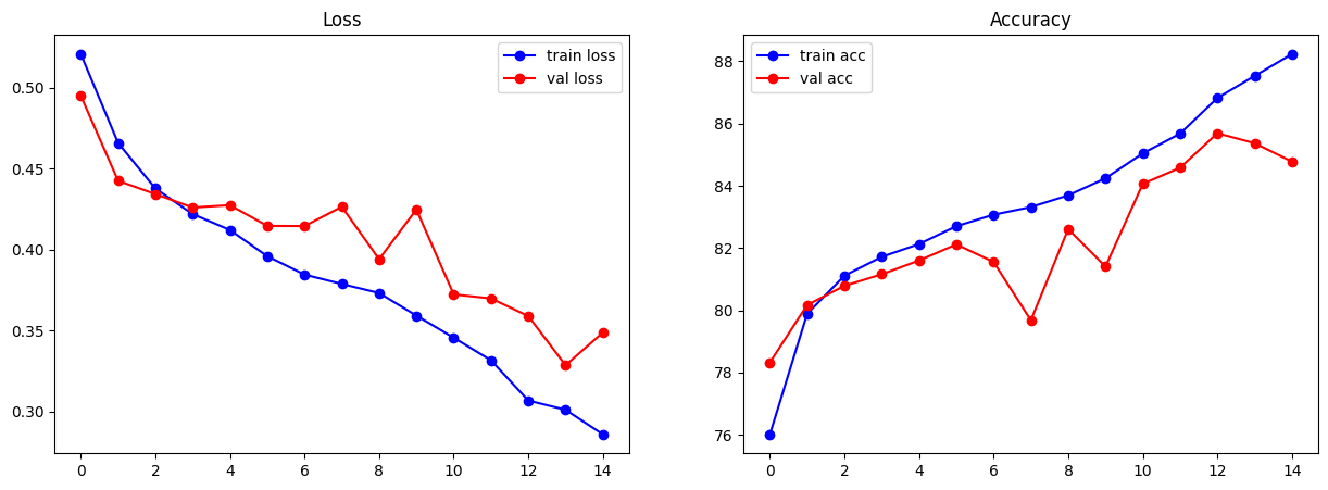
import matplotlib.pyplot as plt

# lets plots the metrics
fig, ax= plt.subplots(nrows = 1, ncols = 2, figsize = (15, 5))
ax[0].plot(metrics_mobileNet['train_loss'], 'bo-', label = 'train loss')
ax[0].plot(metrics_mobileNet['val_loss'], 'ro-', label = 'val loss')
ax[0].set_title('Loss')
ax[0].legend()
ax[1].plot(metrics_mobileNet['train_acc'], 'bo-', label = 'train acc')
ax[1].plot(metrics_mobileNet['val_acc'], 'ro-', label = 'val acc')
ax[1].set_title('Accuracy')
ax[1].legend()
plt.show()
# Lets now test on test data and plot confusion metric as well. Also plot the ROC curve

from sklearn.metrics import confusion_matrix, roc_curve

y_pred = []
y_true = []
with torch.no_grad():
    for inputs, labels in test_loader:
        inputs, labels = inputs.to(device).float(), labels.to(device).float().unsqueeze(1)
        outputs = finetuned_MobileNet_model(inputs)
        y_pred.extend(outputs.cpu().numpy())
        y_true.extend(labels.cpu().numpy())

y_pred = np.array(y_pred)
y_true = np.array(y_true)

# lets compute confusion metric and ROC curve
cm = confusion_matrix(y_true, y_pred > 0.5)
# Plot the confusion matrix
fig, ax = plt.subplots(figsize=(5, 5))
ax.imshow(cm, interpolation='nearest', cmap=plt.cm.Reds)
# put the percentage in each cell
for i in range(cm.shape[0]):
    for j in range(cm.shape[1]):
        ax.text(j, i, f'{cm[i, j]} ({cm[i, j]/np.sum(cm[i, :])*100:.1f}%)', ha='center', va='center', color='white')
ax.set_title('Confusion Matrix')
ax.set_xlabel('Predicted Labels')
ax.set_ylabel('True Labels')

# lets plot the ROC curve
fpr, tpr, _ = roc_curve(y_true, y_pred)
plt.figure(figsize=(5, 5))
plt.plot(fpr, tpr, label='ROC curve')
plt.plot([0, 1], [0, 1], 'k--', label='Random guess')
plt.xlabel('False Positive Rate')
plt.ylabel('True Positive Rate')
plt.title('ROC Curve')
plt.legend()
plt.show()